Financial Markets

Financial markets are not chaos

Introduction

Most retail investors are handed a brokerage account and a login before they are ever handed a map. They are told to buy an index fund, or they are told to chase whatever moved twenty percent last week, and very little in between. The result is a market participant who owns assets without understanding what those assets actually are, who follows strategies without understanding what those strategies are optimized for, and who reacts to headlines without a framework to place them in.

This guide is that map, and it is built to be read two ways: front to back for anyone starting from zero, or as a standing reference to return to whenever a specific concept needs revisiting. It works through the full landscape a retail investor operates in: the asset classes available, the corporate mechanics and events that move an individual stock, how a trade actually moves through the market’s plumbing, how to read a company’s own financial statements and value it properly, the full instrument set from a simple share purchase to a fully specified options strategy, the strategies built around them, the complete technical and macroeconomic toolkit professional desks use, and the portfolio-level discipline that determines whether any of it compounds into a result. It closes with a practical, start-to-finish research process, the mistakes that quietly cost retail investors the most money, and an honest account of why EllTec Analysis builds its own research the way it does.

None of this is a substitute for independent judgement. It is the foundation that judgement is built on.

Part I: The Asset Class Universe

Every portfolio, no matter how sophisticated, is ultimately a combination of a small number of underlying building blocks. Understanding what each one actually represents, and what role it plays, is the first and most neglected step in investing.

Equities

A share of stock is a fractional ownership claim on a company’s assets, earnings, and future cash flows. Equities are the primary engine of long-term wealth creation in a portfolio because they carry a claim on growth itself, but that claim is unsecured and sits behind every creditor in a bankruptcy. Within equities, the split between growth and value, and between large, mid, and small capitalisation, changes the risk and return profile substantially. A mega-cap dividend payer and a pre-profit small-cap growth name are both “stocks,” but they behave like different asset classes entirely. The recurring corporate events that most directly move an individual stock’s price and shape its long-term return, dividends, splits, buybacks, and earnings reports, are covered in full in Part II, and the ownership mechanics behind a share itself, voting rights, free float, and how a trade actually settles, are covered in Part III.

Fixed Income

Bonds are loans. The investor lends capital to a government or a corporation in exchange for a defined coupon and the return of principal at maturity. Fixed income exists in a portfolio primarily to provide ballast, income, and a counterweight to equity volatility, though that relationship is not fixed and has broken down during periods when inflation drives both stocks and bonds lower together. The full mechanics of bond pricing, credit ratings, duration, and the yield curve, along with the money market instruments that sit at the short end of the same universe, are covered in depth in Part VI.

Commodities

Energy, industrial and precious metals, and agricultural products sit outside the financial system in the sense that their value is tied to physical supply and demand rather than a claim on future cash flows. Commodities tend to do best in inflationary, supply-constrained environments and are frequently used as a portfolio hedge against currency debasement. How commodity exposure is actually accessed, and why an investor’s realised return frequently differs from the spot price quoted in headlines, is covered in full in Part XV.

Currencies (FX)

The foreign exchange market is the largest and most liquid market in the world, trading trillions of dollars daily. For most retail investors currencies are not a standalone holding but a background variable that affects the value of every foreign asset they own, and a direct driver of returns for anyone trading internationally. Currency pair mechanics, hedging, and exactly how FX moves change the realised return on a foreign holding are covered in full in Part XIV.

Real Estate and REITs

Property can be owned directly or accessed through Real Estate Investment Trusts, which are listed vehicles that hold income-producing property and are required to distribute the large majority of their taxable income as dividends. REITs offer real estate exposure with equity market liquidity, but they also trade with meaningful correlation to equities and interest rates, particularly because higher rates raise both the cost of financing new property and the discount rate applied to future rental income. Direct property investment is evaluated using its own specific vocabulary, distinct from the securities-based ratios in Part V. Net Operating Income, NOI, is a property’s rental income minus operating expenses, before financing costs and taxes, the real estate equivalent of operating income. The capitalisation rate, or cap rate, is NOI divided by the property’s current market value or purchase price, functioning as real estate’s rough equivalent of an earnings yield: a lower cap rate implies a more expensive property relative to the income it generates, and cap rates across a market compress and expand with interest rates in broadly the same direction described for bond yields in Part VI, since real estate is itself a long-duration, income-generating asset competing for the same capital. Leverage plays an outsized role in direct property returns specifically because financing is so central to how most real estate is actually purchased, and the same operating-leverage logic introduced in Part V applies directly: a modest change in property value or rental income can produce a considerably larger swing in the investor’s actual equity return once mortgage financing is layered underneath it.

Private Equity, Venture Capital, and Private Credit

Beyond the publicly traded markets this guide otherwise focuses on, a substantial pool of capital sits in privately held companies and privately originated loans, entirely outside any stock exchange. Private equity funds acquire established private companies, or take public companies private, typically using significant leverage, with the explicit goal of improving operations and exiting through a sale or a future IPO several years later. Venture capital applies a similar concept to early-stage, high-growth private companies before they are mature enough for a public listing or a private equity buyout, accepting a high failure rate across most individual investments in exchange for the possibility that a small number of successes generate outsized returns for the whole fund. Private credit refers to loans originated directly by non-bank lenders to companies, typically mid-sized businesses that traditional bank lending or the public bond market covered in Part VI does not serve as efficiently, and has grown into a major asset class of its own as banks have pulled back from some forms of corporate lending in recent years. All three have historically been accessible only to institutional investors and accredited individuals able to commit capital for years at a time with no ability to exit early, since the underlying holdings are neither publicly listed nor easily resold. More recent evergreen and interval fund structures have begun opening narrower, still-illiquid retail access to this asset class, and the illiquidity itself, not merely the higher risk of the underlying companies, is the defining feature any retail investor considering this space needs to weigh before committing capital that cannot be recovered on short notice.

Cryptocurrencies

Digital assets are the newest addition to the asset class universe and remain the least settled in terms of valuation framework, regulatory treatment, and correlation behaviour. Bitcoin has increasingly traded as a macro liquidity asset, moving with risk appetite and monetary conditions, while the broader crypto complex still carries idiosyncratic, technology-specific risk on top of that. The asset class is genuinely young. Its correlation to traditional markets has shifted meaningfully over time and should not be assumed to be stable going forward.

The asset class itself is not a single, homogenous thing, and lumping every token into one bucket obscures more than it reveals. Stablecoins are cryptocurrencies pegged to a reference asset, almost always the US dollar, either through fiat and short-term treasury reserves held one-to-one against the tokens in circulation or through an algorithmic or crypto-collateralised mechanism, and they function primarily as the settlement layer and cash-equivalent of the crypto ecosystem rather than as a speculative holding in their own right. A separate category functions as an actual means of payment, using a blockchain’s native token to transfer value directly between parties without a bank or card network intermediary, a use case that has gained the most real-world traction in cross-border remittances and in economies with unstable local currencies. A third category consists of smart contract platforms, which extend beyond simple value transfer to run decentralised applications, lending protocols, and other programmable financial infrastructure directly on the blockchain. Underlying all of this is the consensus mechanism that actually secures the network and validates transactions. Proof of Work, the original mechanism used by Bitcoin, relies on miners competing to solve a computationally expensive puzzle, which secures the network through the sheer cost of the electricity and hardware required to attack it, at the price of substantial energy consumption. Proof of Stake, used by Ethereum since its transition and by most newer networks, replaces that computational race with validators who lock up, or stake, the network’s own token as collateral and are financially penalised for validating fraudulently, achieving comparable security with a small fraction of the energy footprint. The choice of consensus mechanism is not a technical footnote: it shapes a network’s decentralisation, its issuance schedule, and ultimately the investment case for the token that secures it. The trading mechanics specific to this asset class, on-chain activity, perpetual futures, and custody risk among them, are covered in full in Part XVI.

Cash and Money Markets

Cash is the most underrated asset class in a retail portfolio. It carries no market risk, generates yield in a higher rate environment, and represents pure optionality: the ability to deploy capital when opportunities appear rather than being forced to sell something else first. The opportunity cost of holding cash is real, particularly during strong bull markets, but a portfolio with zero cash flexibility is a portfolio that cannot act on its own conviction when it matters most. The specific instruments that make up this asset class are covered alongside fixed income in Part VI.

Part II: Corporate Actions and Company Events

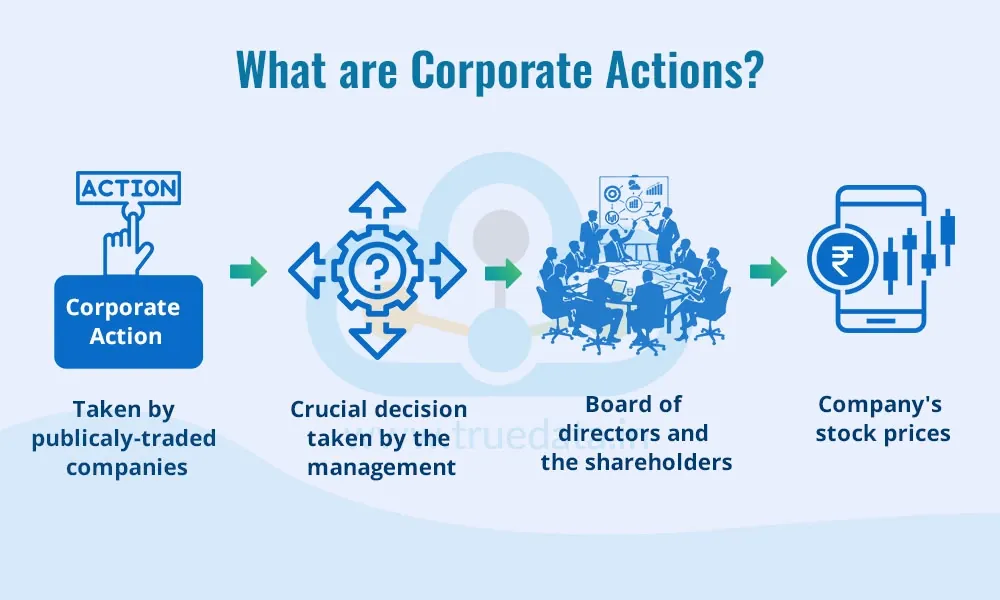
Beyond the asset class itself, individual stocks carry a set of recurring events that materially affect price, ownership, and total return. Understanding the mechanics behind each one prevents a retail investor from being blindsided by a price move that has a perfectly rational, mechanical explanation behind it, rather than a random one.

Dividends

A dividend is the portion of a company’s profit distributed directly to shareholders, most commonly in cash, though occasionally as additional shares in the form of a stock dividend. The mechanism runs through four dates that matter more than most retail investors realise. The declaration date is when the board formally announces the dividend and its amount. The ex-dividend date is the date on or after which a buyer is no longer entitled to the upcoming payment, and the share price mechanically opens lower by roughly the dividend amount on that date, since the cash is effectively leaving the company; this is a structural adjustment, not a sign of weakness. The record date, typically set shortly after the ex-dividend date, is when the company checks its books to confirm exactly who is owed the payment. The payment date is simply when the cash arrives in the shareholder’s account. Two ratios matter for evaluating any dividend: the dividend yield, the annual payment divided by the current share price, and the payout ratio, the dividend divided by earnings, which measures sustainability; a payout ratio pushed close to or beyond one hundred percent signals a dividend that is not comfortably covered by profit and carries elevated risk of being cut. Many brokers offer a Dividend Reinvestment Plan, commonly abbreviated DRIP, which automatically uses the cash payment to purchase additional shares, often without a commission, compounding the position over time with no manual action required. A dividend cut or suspension is one of the more bearish, high-conviction signals a company can send, since management is structurally reluctant to reduce a payment shareholders have come to rely on and typically only does so once cash flow genuinely cannot support it; conversely, a long, unbroken record of raising the dividend year after year signals genuine confidence in the durability of future cash generation. Special dividends, one-off payments made outside the regular schedule, usually follow a windfall event such as an asset sale rather than reflecting ongoing earnings power, and should be read as an isolated event rather than a repeatable one.

Stock Splits and Reverse Splits

A forward stock split increases the number of shares outstanding by a fixed ratio while proportionally reducing the price per share, so that the company’s total market capitalisation and the value of any existing holding are entirely unchanged; a two-for-one split simply turns one share worth a given price into two shares each worth half that price. Companies typically split their stock after a period of strong price appreciation has pushed the nominal share price to a level perceived as psychologically less accessible to smaller investors, and a split is often, though not always, read as a quiet signal of management’s confidence in continued strength. A reverse split runs the same mechanism in the opposite direction, consolidating shares to raise the nominal price, for instance turning ten shares worth a low price each into one share worth ten times as much. Reverse splits are frequently a defensive measure, used to avoid falling below an exchange’s minimum listing price or to make a heavily depreciated stock appear more acceptable to institutional mandates that avoid low nominal share prices, and as such they often follow, and sometimes coincide with, a period of genuinely poor fundamental performance. A reverse split therefore deserves scrutiny of the underlying business rather than being treated as a neutral, cosmetic event.

Share Buybacks

A share buyback is the company itself repurchasing its own stock on the open market, which reduces the number of shares outstanding. The most immediate effect is mechanical: with the same net income now divided across fewer shares, earnings per share rises even if underlying profit has not grown at all, and the ownership percentage of every remaining shareholder increases correspondingly. Buybacks function as an alternative to dividends for returning capital to shareholders, and carry two practical advantages: they can be paused or scaled back without the same negative signal a dividend cut sends, and in many jurisdictions they avoid creating an immediate taxable event for shareholders who choose not to sell. They are not, however, an unambiguous positive. Companies have a well-documented tendency to buy back the most stock when it is expensive, flush with cash during strong periods, and the least when it is genuinely cheap, and a portion of headline buyback activity simply offsets the dilution created by stock-based compensation to employees and executives rather than representing a genuine net return of capital to outside owners. The headline buyback figure is worth checking against the actual share count trend over several years rather than taken at face value.

Earnings Reports

Publicly listed companies report financial results on a recurring cadence, quarterly in the United States and typically semi-annual across many European markets, and the concentrated multi-week window when most companies within an index report is known as earnings season. Two headline figures anchor every report: revenue, the total value of sales, and earnings per share, the profit allocated to each outstanding share. It is worth distinguishing GAAP earnings, calculated under standardised accounting rules, from adjusted or non-GAAP earnings, which management calculates after excluding items it deems one-off or non-operational; adjusted figures can genuinely clarify underlying performance, but they can also be used to flatter results, so it is worth checking both rather than relying on the adjusted number alone. Markets react far less to the absolute figures than to how those figures compare against consensus analyst estimates: a beat is a result above expectations, a miss is a result below them, and a company can report genuine double-digit growth and still see its stock fall sharply if the market had priced in even more. Guidance, management’s forward-looking outlook for the coming quarter or the full fiscal year, is often the single most important element of the entire release, since markets are forward-pricing mechanisms; raised guidance can lift a stock even on an otherwise mixed quarter, while guidance cut lower can hit a stock harder than the quarter’s actual miss did, because it revises the market’s model of future cash flows rather than simply confirming one already-completed period. The earnings call, a scheduled conference call in which management walks through results and takes questions from sell-side analysts, frequently reveals more useful information than the numbers alone, particularly on demand trends, margin trajectory, and competitive positioning. The specific metrics that matter beyond the headline figures vary by sector: subscriber or active user growth for platform businesses, same-store sales for retailers, order backlog or bookings for industrials and software, net interest margin for banks, and checking the metric that actually drives that specific business is often more informative than the top-line beat or miss alone. Price reactions tend to follow two recognisable patterns. Because earnings are typically released outside market hours, the reaction shows up as a gap, a sharp jump or drop at the following session’s open rather than a gradual intraday move, and as post-earnings announcement drift, a well-documented tendency for a stock to keep drifting in the direction of its initial reaction over the following days and weeks as the market continues digesting the release, rather than reverting immediately. For options traders specifically, implied volatility typically inflates heading into a known earnings date in anticipation of the move and then collapses sharply once the event has passed, a dynamic known as volatility crush, which can cause an options position to lose value even when the underlying stock moved in the anticipated direction, if the actual move was smaller than what the elevated premium had already priced in.

Initial Public Offerings

An Initial Public Offering (IPO) is the process by which a private company sells shares to the public for the first time, typically managed by one or more investment banks acting as underwriters, who help set the offering price and allocate the initial tranche of shares, predominantly to institutional investors, ahead of the public listing. Early insiders, founders, employees, and pre-IPO investors are almost always bound by a lock-up period, commonly ninety to one hundred and eighty days, during which they are contractually restricted from selling their shares; the lock-up expiration date is itself a well-known and often-anticipated event, since a wave of previously restricted shares becoming sellable at once can create meaningful selling pressure regardless of how the underlying business is performing. Newly listed stocks tend to carry outsized volatility in their first weeks and months of trading, driven by a limited public float, unsettled price discovery, and the absence of a long trading history or an established investor base to anchor valuation. It is also worth noting plainly that retail investors typically only gain access at the public listing price, while the discounted allocation price offered to institutional investors ahead of the listing is rarely available to them, which is part of why a stock can open, and sometimes remain, well above the price institutional buyers actually paid.

Capital Raises: Rights Offerings, Follow-on Offerings, and Private Placements

A rights offering gives existing shareholders the right, but not the obligation, to buy additional shares, usually at a discount to the market price, in proportion to their existing holding, and exists primarily to raise capital without forcing a company through a broker-negotiated placement; a shareholder who does not participate is diluted, since new shares are created without that shareholder’s own stake growing to match. A secondary or follow-on offering is a company selling additional new shares to the market after its IPO, typically increasing shares outstanding and diluting existing holders, and the market’s reaction depends heavily on the stated purpose, whether the capital is funding growth or plugging a balance-sheet hole. An At-The-Market, or ATM, offering is a more gradual version of the same mechanism, where a company sells new shares incrementally into the existing trading market over time rather than in one large discrete block, which spreads the dilutive impact but can create a persistent overhang on the share price as the market anticipates ongoing supply. A private placement sells new shares or debt directly to a small number of institutional or accredited investors outside the public market, usually faster and cheaper to execute than a public offering but often priced at a discount that dilutes existing shareholders more per dollar raised.

Convertible Debt and Tender Offers

Convertible debt is a bond that gives the holder the option to convert it into a predetermined number of shares, combining a bond’s downside protection, its coupon and principal, with equity-like upside if the share price rises past the conversion price. Companies issue convertible debt to raise capital at a lower coupon than a straight bond would require, in exchange for giving bondholders that upside optionality, which is itself a form of future dilution worth tracking. A tender offer is a public invitation, from the company itself as a buyback tender or from an outside acquirer, to purchase shares directly from shareholders at a stated price, usually at a premium to the market price, within a defined window, and is a faster mechanism for a large ownership change than accumulating shares gradually on the open market.

Mergers, Acquisitions, and Corporate Restructuring.

A merger combines two companies into one, while an acquisition sees one company purchase and absorb another, and in both cases the target’s shareholders typically receive cash, acquirer shares, or a combination, at a premium to the pre-announcement price that reflects the value of control and expected synergies. A spin-off separates an existing division into its own independently listed company, with shares typically distributed pro-rata to existing shareholders of the parent, done when the market is judged likely to value the two businesses more highly apart than combined, a dynamic sometimes described as removing a conglomerate discount. A carve-out is similar but sells only a minority stake of the division to the public while the parent retains control, and a divestiture is an outright sale of a division to another company or private buyer rather than a public listing. A Special Purpose Acquisition Company, or SPAC, is a shell company that lists on an exchange with no underlying operating business, raises capital, and then has a defined window to merge with a private company, effectively taking that company public through the back door rather than a traditional IPO; SPACs carry a distinct risk profile, since the eventual merger target is often unknown at the time of the initial listing, and the share price can swing heavily on merger rumours and eventual deal terms. Delisting removes a company’s shares from an exchange, either voluntarily, through a takeover or a decision to go private, or involuntarily, through failure to meet listing standards such as a minimum share price or market capitalisation, and involuntary delisting typically forces the stock into much less liquid over-the-counter trading. Bankruptcy protection, Chapter 11 reorganisation in the US being the most referenced example, allows a company to continue operating while restructuring its debts under court supervision, and in the large majority of cases existing common equity is wiped out or reduced to a small fraction of its former value, since creditors are repaid before shareholders in the legal priority of claims. A share cancellation permanently retires repurchased shares rather than holding them as treasury stock, which locks in the EPS-accretive effect of a buyback described above.

Insider Transactions and Activist Investors

Insider buying and selling, transactions by a company’s own executives and directors in its shares, must be publicly disclosed in most developed markets and is watched as a signal, though asymmetrically: insider selling is common and often driven by ordinary diversification or tax-planning needs, while insider buying, particularly cluster buying by multiple executives at once, is a comparatively rarer and more information-dense signal, since an executive has no routine, non-signalling reason to add to a position with personal capital. An activist investor is typically a fund that accumulates a meaningful stake in a company specifically to push for change, whether operational, strategic, or in the makeup of the board, and a proxy fight is the formal mechanism by which an activist solicits other shareholders’ votes to support its proposed slate of directors or resolutions against management’s own recommendation at the annual shareholder meeting. The presence of an activist stake is itself often treated as a catalyst, since it signals that someone with capital at risk and genuine influence believes the company is undervalued or mismanaged.

Index Inclusion, Exclusion, and Rebalancing

Major indices such as the S&P 500 are not static; they are periodically reconstituted, with companies added or removed based on defined criteria including market capitalisation, liquidity, and profitability. Addition to a widely tracked index creates genuine, mechanical buying pressure, since every index fund and ETF tracking that benchmark must purchase the new constituent to maintain its tracking accuracy, and removal creates the mirrored, mechanical selling pressure; this is a structural, flow-driven price effect that is largely independent of any change in the company’s actual fundamentals. Periodic rebalancing, even without an addition or removal, adjusts each existing constituent’s weight to match the index’s methodology, which is why heavily tracked indices can see concentrated trading volume around known rebalancing dates.

Part III: Market Structure, How a Trade Actually Happens

Understanding what an asset is and what moves it is only half the picture. The other half is the plumbing: what actually happens between deciding to buy something and owning a settled position, and the mechanics that quietly determine the price an investor actually receives versus the price they saw quoted.

Primary and Secondary Markets

The primary market is where a security is sold for the first time, an IPO or a new bond issuance, and the capital raised goes directly to the issuing company or government. Every trade after that happens in the secondary market, where capital simply changes hands between investors and the issuer receives nothing further. Nearly everything a retail investor does day to day happens in the secondary market; the primary market is the exception, not the rule.

Exchanges and Over-the-Counter Markets

An exchange is a centralised, regulated venue, such as the NYSE, Nasdaq, or Deutsche Börse’s Xetra, where orders are matched against a public, visible order book under a standard rulebook. Over-the-counter, or OTC, trading happens bilaterally between two parties, or through a dealer network, without a centralised order book, and is common for most bonds, many structured products such as the certificates covered in Part VII, and smaller or less liquid stocks. OTC trading is generally less transparent on price and carries more counterparty-specific risk than an exchange-matched trade.

ADRs and GDRs

Buying a foreign company’s shares does not always mean trading directly on its home exchange. An American Depositary Receipt, ADR, is a US-listed certificate representing shares of a foreign company, issued by a US depositary bank that holds the actual foreign shares in custody and issues a dollar-denominated, US-exchange-tradable receipt against them, letting a US investor buy and sell that foreign company through an ordinary US brokerage account, in dollars, without opening a foreign trading account or dealing with a foreign exchange’s own settlement conventions directly. A Global Depositary Receipt, GDR, is the same basic structure used more broadly to list a company’s shares on exchanges outside its home market, commonly used to raise capital in London or other international financial centres. ADRs come in different levels reflecting how much regulatory disclosure the foreign company has taken on: unsponsored and lower-level sponsored ADRs trade over-the-counter with limited reporting, while higher-level sponsored ADRs list on a major exchange such as the NYSE or Nasdaq and carry the same disclosure standards as a domestic listing. Crucially, an ADR does not eliminate the FX exposure covered in Part XIV, since the depositary bank converts the underlying foreign dividend and any corporate action proceeds into dollars at the prevailing exchange rate; what it removes is the operational friction of trading directly on a foreign exchange, not the currency risk itself. An ADR ratio determines how many underlying foreign shares each ADR represents, which can be one-to-one or a different multiple entirely, and is worth checking before comparing an ADR’s price directly against the foreign share’s own home-market price.

Dark Pools

Not all trading happens on a visible, public order book. A dark pool is a private trading venue where buy and sell orders are matched without displaying that order interest publicly beforehand, used predominantly by institutional investors to execute large orders without revealing their intentions to the wider market ahead of time, which would otherwise move the price against them before the full order could be filled, precisely the market impact problem described below. Trades executed in a dark pool are still reported to the public tape after execution, so the trade itself becomes visible in hindsight, but the order that produced it was never visible in advance the way a resting order on a lit exchange’s order book would be. Dark pools now account for a meaningful share of total trading volume in major markets, and their existence is part of why the order book depth visible on a public exchange does not represent the full picture of actual supply and demand at any given moment, a genuinely important caveat to the price discovery and market depth concepts introduced below.

Market Makers and Liquidity Providers

A market maker continuously posts both a bid and an ask for a given security, providing the liquidity that lets other participants trade immediately rather than waiting for a natural counterparty to appear, and earns the bid-ask spread as compensation for that service and the risk of holding inventory. Some exchanges formally designate market makers with obligations to maintain a two-sided quote within defined limits; a broader universe of liquidity providers, including high-frequency trading firms, perform a similar function without a formal designation. Without this layer, a retail market order in a thinly traded name could sit unfilled indefinitely.

Brokers, Clearing Houses, and Custodians

These three roles are frequently conflated by retail investors and are worth separating clearly. The broker is the intermediary that receives an order and routes it to the market for execution; it does not itself hold the investor’s assets in the sense of legal ownership. The clearing house sits between the buyer and the seller after a trade is agreed, a process called novation, becoming the counterparty to both sides and guaranteeing the trade will settle even if one of the original parties defaults, which is what removes bilateral counterparty risk from everyday trading. The custodian is the entity that actually holds and administers the securities on behalf of the owner, whether that is the broker itself, a sub-custodian bank, or a central securities depository, and this distinction becomes directly relevant to broker-risk questions covered in Part XVIII.

Settlement, T+1 and T+2

A trade is agreed on the trade date, but ownership and cash do not legally change hands until the settlement date, days later. The US market moved to a T+1 standard, meaning settlement one business day after the trade; many European markets still operate on T+2. This gap matters because it defines the window during which counterparty risk exists between agreement and final settlement, and it also explains why the ex-dividend date mechanics covered in Part II are set the way they are, since entitlement to a dividend is determined by who is the settled owner of record on a specific date, not simply who placed a buy order before it.

The Order Book, Bid-Ask Spread, and Market Depth

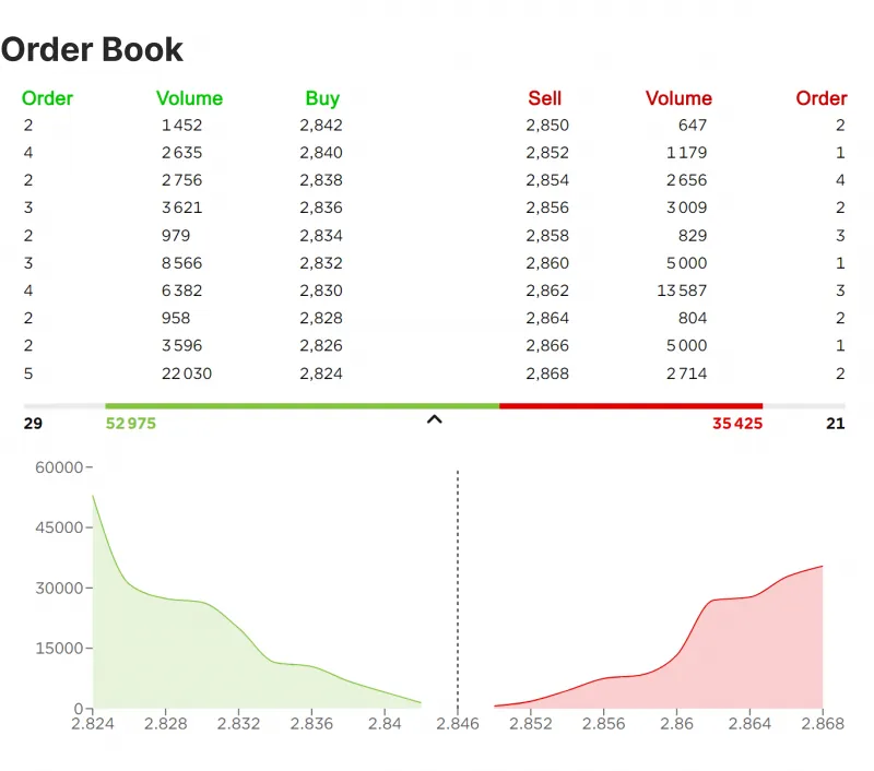
The order book is the real-time, price-ranked list of every resting buy order (bid) and sell order (ask) for a given security. The bid-ask spread, the gap between the best available bid and the best available ask, is the implicit cost of trading immediately rather than waiting, and it widens or narrows directly with a security’s liquidity: a mega-cap stock might trade on a spread of a fraction of a cent, while a thinly traded small-cap or an out-of-the-money option can carry a spread worth a meaningful percentage of the price itself. Market depth describes how much order size sits at each price level beyond just the best bid and ask; shallow depth means a moderately sized order can “walk the book,” consuming several price levels and receiving a progressively worse average price, which is the direct mechanism behind both of the next two concepts.

Slippage and Market Impact

Slippage is the gap between the price an investor expected when placing an order and the price actually received on execution, driven by the time between decision and fill, by order type (a market order accepts whatever the book currently offers, exactly as described in the Order Types entry in Part IV), and by how much size is being traded relative to available depth. Market impact is the closely related concept of the trade itself moving the price, relevant mainly for larger orders relative to a security’s typical volume, and it is the reason institutional desks break large orders into smaller pieces over time rather than executing all at once, and part of why the liquidity heatmaps covered later in this guide are watched as a proxy for where that impact is likely to be smallest or largest.

Price Discovery

Price discovery is the continuous process by which the interaction of all resting and incoming buy and sell orders arrives at a market-clearing price reflecting all currently available information. This is, in the most literal sense, what “the market” is doing at every moment a security trades, and it is why a stock’s price can move meaningfully on light volume when very little new information has actually changed hands: the order book itself is thin enough that even modest new flow shifts where that clearing price sits.

Trading Halts and Circuit Breakers

Individual stocks can be halted from trading, most commonly pending material news that has not yet been fully disseminated, or automatically, on some exchanges, when the price moves beyond a defined percentage within a short window. Circuit breakers operate at the market-wide level, automatically pausing trading across an entire exchange when a benchmark index falls by a defined percentage within the session. Both mechanisms exist for the same underlying reason: to create a deliberate pause that gives participants time to absorb information and reassess, rather than allowing a self-reinforcing, momentum-only cascade to run unchecked.

Opening and Closing Auctions

Rather than matching orders continuously, most exchanges determine the official opening and closing price through a batch auction, which aggregates all buy and sell interest submitted for that specific auction and calculates the single price that clears the maximum possible volume. This concentrates an enormous amount of trading into a very short window, which is why closing-auction volume is frequently the single largest print of the trading day, and why volume can spike sharply around known index rebalancing dates, directly tying back to the mechanical flows described in Part II.

Pre-Market and After-Hours Trading

Trading that happens outside the standard session, before the open or after the close, operates with meaningfully thinner liquidity and wider spreads than the regular session, since far fewer participants and market makers are active. This is directly relevant to the earnings reaction dynamics covered in Part II, since earnings are typically released outside market hours and the market’s first, often outsized, reaction plays out in this comparatively illiquid window before the full session reopens.

Institutional Versus Retail Order Flow

Institutional order flow, from pension funds, mutual funds, hedge funds, and other large managers, tends to be larger per trade, more research-driven, and more price-impactful than the typical retail order. In several major markets, a substantial share of retail order flow is routed through arrangements where market makers pay brokers for the right to execute that flow directly, known as payment for order flow, rather than sending it straight to a public exchange; this remains a source of ongoing regulatory scrutiny in some jurisdictions and is worth being aware of as a structural feature of how a “commission-free” retail trade is actually monetised.

Equity Ownership Mechanics

Common shares carry voting rights and a residual, variable claim on earnings; preferred shares typically carry a fixed dividend with priority over common dividends but usually no voting rights, functioning as a hybrid between a bond and an equity. Voting structures are not always one-share-one-vote: dual-class share structures, where one class carries substantially more votes per share than another, exist specifically to let founders or early insiders retain control while still raising public capital. Shares outstanding is the total number of shares a company has issued; free float excludes shares held by insiders, strategic holders, or under lock-up, and represents what is actually available for public trading, which matters because a low free float relative to total shares outstanding can produce outsized volatility on relatively modest trading volume. Treasury shares are shares the company has repurchased and continues to hold itself rather than cancelling, and are excluded from the shares-outstanding count used for EPS purposes, distinguishing them from the cancellation event described in Part II. Institutional ownership, the percentage of shares held by funds and other large managers, and insider ownership, the percentage held by executives and directors, are both tracked as rough proxies for conviction and also affect a stock’s practical liquidity. Shares held in a standard brokerage account are frequently lent out by the broker to short sellers in exchange for a fee, a normal, regulated practice that is part of how the short-selling mechanism described in Part IV is actually sourced; the broker-level implications of this practice are covered further in Part XVIII. Finally, dilution, any increase in shares outstanding that reduces each existing shareholder’s proportional ownership, is not limited to the capital raises covered in Part II; stock-based compensation to employees and executives is a major and frequently under-appreciated source of ongoing dilution in its own right, a point picked up again in the earnings-quality discussion in Part V.

Part IV: How Retail Investors Actually Access These Markets

Owning the asset class is one question. The instrument used to get that exposure is a separate question, and the choice of instrument changes the risk profile considerably even when the underlying exposure looks the same on paper.

Direct share and bond purchase

Buying an individual stock or bond outright gives full, uncomplicated ownership with no counterparty layered in between, no expiry date, and no financing cost. It also concentrates risk in a single name unless deliberately diversified across many positions.

Exchange-Traded Funds (ETF)

ETFs bundle a basket of underlying assets into a single, exchange-listed security and are covered in full in Part VIII, because they deserve a dedicated and honest treatment rather than a passing mention.

Mutual Funds

Actively or passively managed pooled vehicles that price once per day rather than trading continuously through the session. They typically carry higher fees than comparable ETFs and often include minimum investment thresholds, but remain common inside retirement and pension structures.

Robo-Advisors

Automated portfolio management services that build and periodically rebalance a diversified portfolio, typically constructed from the low-cost ETFs covered in Part VIII, based on an investor’s stated risk tolerance and goals gathered through an onboarding questionnaire. They offer a lower-cost, more hands-off alternative to traditional discretionary wealth management, and some incorporate automated tax-loss harvesting, the technique introduced in Part XVIII, directly into their ongoing management. The tradeoff is standardisation: a robo-advisor’s allocation logic is necessarily rules-based and generalised across many clients with a similar stated risk profile, rather than genuinely personalised to an individual’s full financial picture the way an ongoing human advisory relationship can be.

Options

A call option gives the buyer the right, but not the obligation, to purchase an asset at a fixed strike price before expiry; a put option gives the right to sell. Options allow an investor to define risk precisely, to generate income against existing holdings, or to take a leveraged directional view with a known maximum loss when buying rather than selling them. They are also decaying assets: time works against the option buyer every single day, which is the single most important thing a new options trader needs to internalise before risking capital. The complete mechanics, including the Greeks and the standard strategy set, are covered in full in Part VII.

Futures

Standardised contracts obligating the buyer to purchase, and the seller to deliver, an asset at a set price on a future date. Futures are used heavily in commodities, indices, and currencies, and are inherently leveraged instruments because only a fraction of the contract’s notional value is posted as margin. That leverage cuts both ways with equal force. Contract mechanics, margin, and the futures curve are covered in full in Part VII.

CFDs and Leveraged Certificates

Contracts for Difference (CFD) and structured products such as Optionsscheine and Knock-Out Zertifikate, instruments widely marketed to retail investors across European markets, allow exposure to an asset’s price movement without owning the underlying asset itself, typically with embedded leverage. These products can be useful for short-term, tactically defined trades, but the leverage embedded in them means that a routine market move can produce an outsized, sometimes total, loss of the capital committed. Regulators across Europe have repeatedly flagged that the large majority of retail accounts trading CFDs lose money, and that statistic should be treated as a serious warning rather than background noise. The full structured-products landscape, including why two products both marketed as identical leverage can carry very different risk, is covered in Part VII.

Margin Trading

Borrowing capital from a broker to increase position size beyond what cash alone would allow. Margin amplifies gains and losses symmetrically and introduces the risk of a forced liquidation, a margin call, at exactly the moment when the position has already moved against the investor and prices are least favourable to sell into.

Short Selling

Selling a borrowed asset with the intention of buying it back later at a lower price, returning the borrowed shares to the lender and pocketing the difference. Short selling inverts the normal risk profile of investing: a long position’s maximum loss is capped at the capital committed, since a price cannot fall below zero, while a short position’s theoretical loss is unlimited, since there is no ceiling on how high a price can rise before the position must eventually be bought back. Short sellers also pay an ongoing borrowing fee to the share lender, which rises sharply when a stock is heavily shorted and hard to borrow, and remain exposed to a short squeeze, a rapid, self-reinforcing price spike that forces short sellers to buy back their position at a loss, with that very buying adding further upward pressure to the price. The aggregate level of short interest in a stock, the percentage of its available float currently sold short, and days-to-cover, that float expressed as a multiple of average daily volume, are tracked as sentiment indicators and, when unusually elevated, as a warning sign for exactly this kind of squeeze dynamic, a point revisited in Part XII.

Order Types

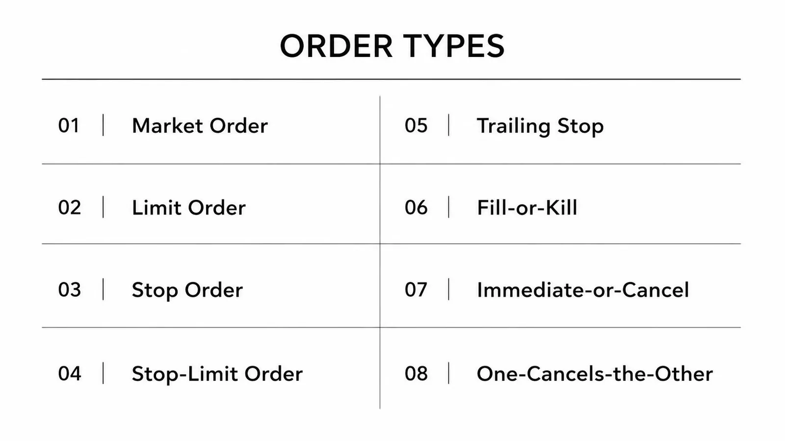
How a trade is executed matters just as much as the decision to make it. A market order executes immediately at the best price currently available, guaranteeing execution but not price, which makes it efficient in liquid markets and dangerous in thin or fast-moving ones where the fill can land well away from the last quoted price, the slippage phenomenon described in Part III. A limit order does the opposite: it only executes at a specified price or better, guaranteeing price but not execution, since the market may simply never trade there. A stop order, commonly used as a stop-loss, sits dormant until a trigger price is reached and then converts into a market order, which protects against catastrophic loss but can still fill at a materially worse price than the trigger during a sharp gap or a flash move. A stop-limit order narrows that risk by converting into a limit order rather than a market order once triggered, at the cost of potentially not filling at all if price moves straight through the limit level without pausing. A trailing stop automatically ratchets the stop level in the direction of a favourable move, locking in gains progressively while leaving the position open to further upside.

Beyond the order type itself, time-in-force instructions determine how long an order remains live: a day order expires unfilled at the end of the session, while a good-till-cancelled order stays active until it either fills or is manually withdrawn. Fill-or-kill and immediate-or-cancel orders demand instant execution, in full or in part respectively, and cancel whatever cannot be filled at once, a structure typically reserved for larger or time-sensitive orders. A one-cancels-the-other order pairs a profit target and a stop-loss around a single position so that the execution of either one automatically cancels the other, which is the simplest and most disciplined way to bracket a trade with defined risk on both sides from the moment it is opened.

The instrument is never a neutral wrapper. The same directional view on the same asset can be expressed with radically different risk depending on whether it is taken through a direct share purchase, a long-dated call option, or a five-times-leveraged CFD.

Part V: Fundamental Analysis and Valuation

Every ratio EllTec Analysis reports, P/E, ROE, margins, leverage, comes from somewhere. This Part is where those numbers actually originate and how to read them properly, so that a ratio quoted elsewhere in this guide or in any EllTec report is never just a number taken on faith.

The Financial Statements

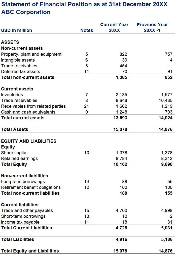
A public company reports four statements every period, and each answers a different question. The income statement answers “did the business make money this period,” running from revenue down through cost of goods sold to gross profit, then operating expenses to arrive at operating income (also called EBIT), then interest and tax to arrive at net income, the bottom line. EBITDA, earnings before interest, tax, depreciation, and amortisation, adds the non-cash depreciation and amortisation charges back to EBIT and is widely used as a rough proxy for a business’s pre-capital-expenditure cash generation, though it is not a cash flow measure itself and can flatter capital-intensive businesses that must reinvest heavily just to stand still. The balance sheet answers “what does the business own and owe right now,” a snapshot rather than a period, built on the identity that assets always equal liabilities plus shareholders’ equity. Assets and liabilities are each split into current (convertible to cash or due within a year) and non-current, and the gap between current assets and current liabilities is working capital, a direct measure of short-term operating liquidity. The cash flow statement answers “where did the actual cash go,” split into operating (cash generated by the core business), investing (capital expenditure and acquisitions), and financing (debt issuance or repayment, dividends, buybacks) activities, and it exists precisely because net income and cash are not the same thing under accrual accounting, covered next. The statement of shareholders’ equity tracks everything that changed a company’s book equity over the period: retained earnings, new share issuance, buybacks, and stock-based compensation all flow through it. The four statements connect: net income from the income statement flows into retained earnings on the equity statement and is the starting point for the cash flow statement’s operating section; the ending cash balance on the cash flow statement matches the cash line on the balance sheet.

Accounting Concepts That Make Ratios Interpretable

Revenue recognition determines when a sale actually counts as revenue, which is not necessarily when cash is received; a software company billing annually in advance recognises that revenue gradually over the service period, not all at once, which is why deferred revenue, cash already collected for a service not yet delivered, sits as a liability on the balance sheet rather than being immediately counted as profit. This is the essence of accrual accounting, which records economic activity when it occurs rather than when cash physically moves, and it is precisely why net income can diverge meaningfully from operating cash flow. Depreciation spreads the cost of a physical asset over its useful life rather than expensing it all at purchase; amortisation does the same for intangible assets. Goodwill is the premium paid in an acquisition above the fair value of the target’s identifiable net assets, sits on the balance sheet indefinitely rather than being amortised, and must be tested periodically for impairment, a write-down taken when the acquired business is no longer worth what was paid for it, which is a direct, honest admission that a prior capital allocation decision did not work out. Working capital components deserve individual attention: accounts receivable is money owed by customers who have already been billed; inventory is unsold goods; accounts payable is money owed to suppliers. Rising receivables or inventory growing meaningfully faster than revenue is a classic early red flag, covered further below. Deferred taxes arise from timing differences between how income is recognised for accounting purposes versus tax purposes and generally even out over time rather than representing a genuine ongoing cash item.

Profitability Ratios

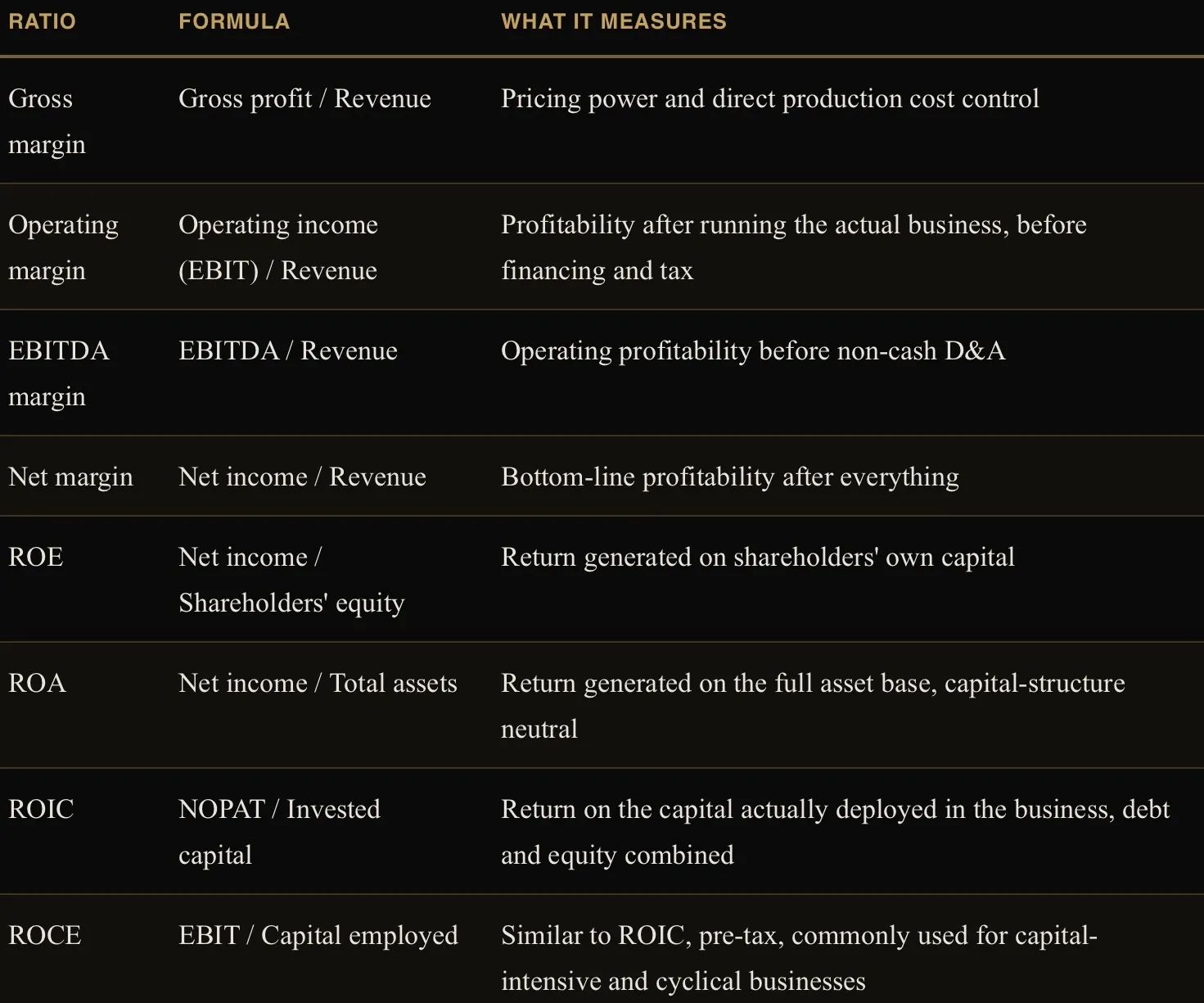
ROE can be flattered by leverage alone, since a highly indebted company can post a high ROE on a shrunken equity base without the underlying business being especially good, which is exactly why ROIC, which is capital-structure neutral, is the more reliable test of whether a business genuinely earns attractive returns on the capital it deploys. The single most useful context for any of these figures is the company’s own trend over several years and its position relative to direct sector peers; a 15% operating margin is unremarkable for a software company and exceptional for a grocery retailer.

Cash Flow Quality

Operating cash flow strips out the non-cash accounting items on the income statement to show cash actually generated by the core business. Capital expenditure, spending on property, plant, and equipment needed to maintain or grow the business, is subtracted from operating cash flow to arrive at free cash flow, the cash genuinely available to shareholders and creditors after the business has reinvested in itself. Free cash flow yield, FCF divided by market capitalisation or enterprise value, is often a more honest valuation anchor than earnings-based multiples precisely because it cannot be distorted by non-cash accounting choices the way net income sometimes can. Cash conversion, operating cash flow divided by net income, run consistently below one signals that reported profit is not fully translating into cash, worth investigating rather than dismissing.

Leverage and Solvency

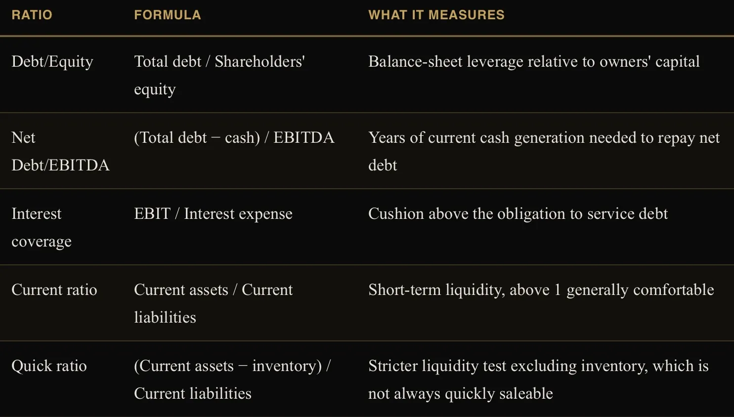
A net cash position, cash exceeding total debt, effectively makes Net Debt/EBITDA negative and is a meaningful sign of balance-sheet flexibility, particularly valuable heading into a downturn or a period of rising rates.

Earnings Quality and Red Flags

Reported earnings are not automatically the same thing as economic reality, and a handful of checks catch most of the difference. Stock-based compensation is a genuine, real economic cost to existing shareholders through the dilution it eventually causes, even though it is a non-cash expense that many companies exclude from their adjusted, non-GAAP earnings figures; a valuation built entirely on an SBC-excluded earnings number is systematically too generous. Receivables or inventory growing consistently faster than revenue can indicate channel-stuffing (pushing sales to distributors that have not actually sold through to end customers) or genuine demand weakness being masked. Frequent “one-time” or “non-recurring” charges that recur every single year are, definitionally, not actually one-time, and should be added back to true underlying earnings only with real skepticism. A balance sheet where goodwill and intangibles make up a large share of total assets is one where a future impairment is a live, real risk rather than a remote one. None of these are automatic disqualifiers, but each is worth a specific, deliberate check rather than being waved through.

Operating Leverage, Competitive Position, and Capital Allocation

Operating leverage describes how much a company’s fixed versus variable cost structure amplifies the swing in profit for a given swing in revenue; a business with high fixed costs and low variable costs sees profit grow (or shrink) far faster than revenue itself once volume crosses its break-even point, which is why airlines and software companies alike can look dramatically more or less profitable across a cycle despite comparatively modest revenue changes. A durable competitive advantage, commonly called a moat, is what protects a business’s returns from being competed away over time, and takes a handful of recognisable forms: network effects (the product gets more valuable as more people use it), switching costs (customers face real friction leaving), a structural cost advantage, brand and intangible value, or efficient scale in a market too small to support a second competitor profitably. Total addressable market, the total revenue opportunity available if a company captured its entire relevant market, is a useful sanity check on how much room a growth story genuinely has left, and pricing power, the ability to raise prices without losing proportional volume, is one of the most direct real-world tests of whether a moat is genuine or merely assumed. Capital allocation, how management chooses to deploy the cash the business generates between reinvestment, acquisitions, debt paydown, dividends, and buybacks, is arguably the single most important and most under-scrutinised judgement a management team makes, and the clearest test of its quality over time is simply whether ROIC has been sustainably above the company’s cost of capital, WACC (Weighted Average Cost of Capital), covered next.

Valuation: The Multiples Framework

Enterprise value, market capitalisation plus total debt minus cash, represents the total cost of acquiring the entire business including its debt, and is the correct numerator for comparing companies with different capital structures, which is why EV-based multiples are generally preferred over equity-only multiples like P/E when comparing across a sector with varying leverage.

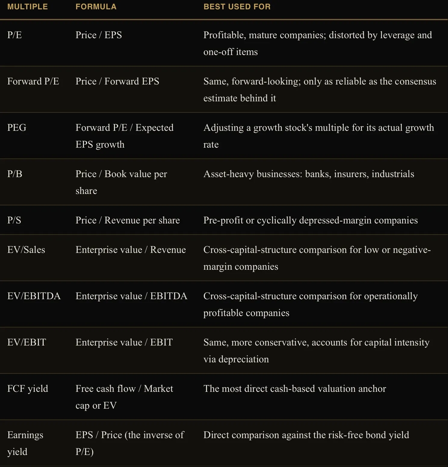
A high P/E is not automatically expensive, and a low P/E is not automatically cheap, and treating either as a mechanical rule is one of the most common analytical errors a retail investor makes. A high multiple can simply reflect a market correctly pricing in genuinely superior future growth, higher quality and durability of earnings, or lower risk, in which case it is not “expensive” so much as a fair price for a better business; conversely, a low multiple frequently reflects a market correctly pricing in declining earnings, elevated financial or business risk, or genuine structural decline, in which case it is not “cheap” so much as an accurate reflection of a deteriorating outlook, precisely the trap value investing (Part IX) explicitly warns against. The only way to actually answer whether a multiple is justified is to compare it against the company’s own growth rate (the logic behind PEG), its own trailing history, and its direct sector peers, never in isolation.

Intrinsic Valuation

A Discounted Cash Flow, or DCF, model estimates a company’s value directly from its expected future cash generation rather than from what other companies happen to trade at. The mechanism: project free cash flow forward for an explicit forecast period, typically five to ten years, discount each year’s cash flow back to today’s value using the Weighted Average Cost of Capital, WACC, then estimate a terminal value representing everything beyond the explicit forecast, either via a perpetual growth rate (the Gordon Growth model) or an exit multiple applied to the final forecast year, discount that terminal value back to today as well, and sum everything to arrive at enterprise value; subtracting net debt gives equity value, and dividing by shares outstanding gives a per-share intrinsic value estimate. WACC blends the cost of equity, commonly estimated via the Capital Asset Pricing Model as the risk-free rate plus the company’s beta multiplied by the equity risk premium, and the after-tax cost of debt, weighted by their respective shares of the capital structure; a higher WACC discounts future cash flows more heavily and produces a lower valuation, all else equal, which is exactly the mechanism through which the interest-rate sensitivity described in Part VI transmits into equity valuations. Because a DCF’s output is highly sensitive to the terminal growth assumption and the discount rate, sensitivity analysis, rerunning the model across a reasonable range of both inputs rather than relying on a single point estimate, is not optional; a DCF that only shows one output number is a DCF hiding its own uncertainty. A reverse DCF flips the exercise: instead of solving for a fair value given assumed growth, it solves for the growth rate the current market price already implies, which is often a faster and more honest way to judge whether a valuation is reasonable, since it removes the analyst’s own growth assumption from the equation entirely. Sum-of-the-parts valuation values a multi-segment or conglomerate business by valuing each division separately, using the multiple appropriate to that specific division’s industry, and summing the results, frequently used to test whether a company might be worth meaningfully more broken apart, the same logic that drives the spin-off decisions covered in Part II.

Relative and Market-Wide Valuation

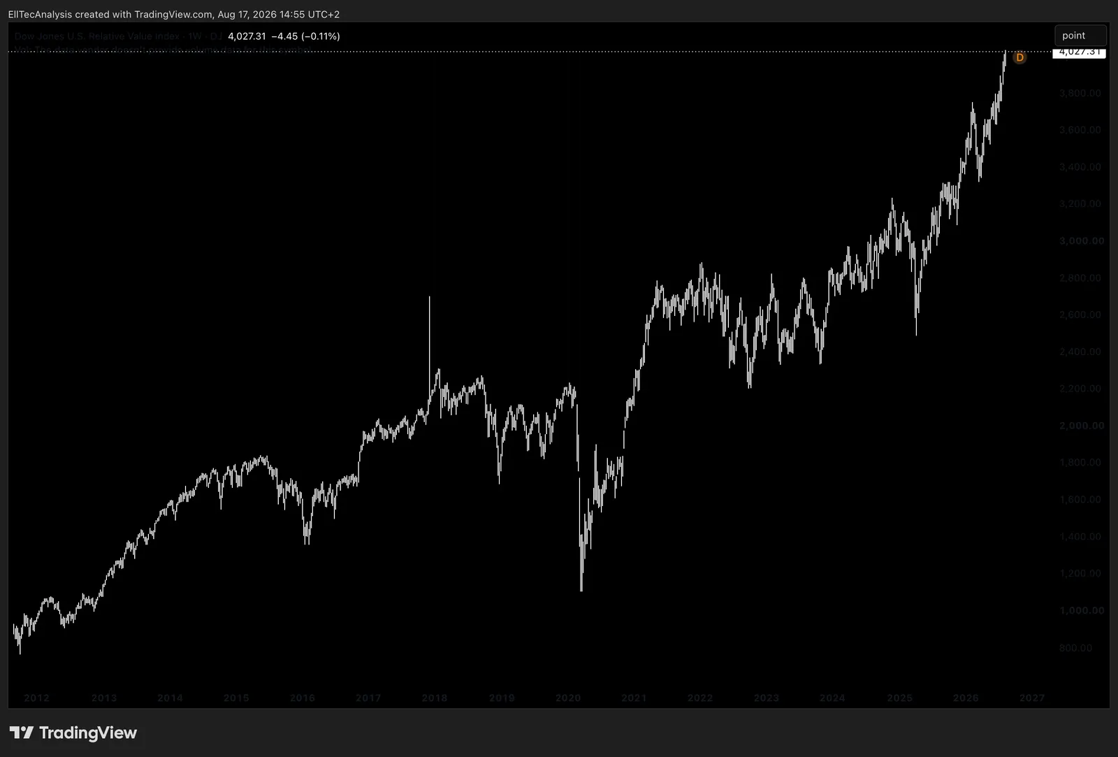
Absolute valuation (DCF) estimates intrinsic worth independent of what anything else trades at; relative valuation (multiples) estimates worth by comparison to peers, the sector, or the company’s own history, and the two approaches are complementary checks on each other rather than substitutes. Historical valuation compares a company’s current multiple to its own trading range over recent years, useful context but not proof of anything on its own, since the business or its growth outlook may have genuinely and permanently changed. Peer and sector valuation compares a company against direct competitors and the broader sector average, the most common practical shortcut, with the important caveat that an entire sector can be simultaneously overvalued or undervalued, so being “cheap relative to peers” is not the same as being cheap in an absolute sense. Market-wide valuation extends the same logic to an entire index, commonly expressed as the market’s aggregate earnings yield compared against the prevailing government bond yield, the equity risk premium, the excess return equities are expected to deliver over a risk-free bond for taking on additional risk; a compressed equity risk premium signals that stocks are priced expensively relative to bonds, and vice versa. Multiple expansion, a rising valuation multiple, and multiple contraction, a falling one, can drive a stock’s return independently of, and sometimes in direct opposition to, its underlying earnings growth, which is the mechanism behind the growth-versus-valuation tradeoff already introduced via PEG: a company can grow earnings twenty percent a year and still produce a poor stock return if its multiple contracts by more than that over the same period, and the reverse is equally true.

ESG and Sustainable Investing

Beyond the traditional fundamental lens covered above, a growing share of research and capital applies an Environmental, Social, and Governance (ESG) framework, scoring companies on factors such as carbon footprint and resource use, labour practices and supply chain conduct, and board independence and executive accountability, alongside or instead of traditional financial metrics. Green bonds, debt instruments where the proceeds are contractually earmarked for environmentally beneficial projects, and ESG-labelled equity funds and ETFs are the most common ways retail investors actually access this approach in practice. The honest caveat worth stating plainly: ESG ratings vary considerably between rating providers, since no single, universally agreed methodology exists for scoring a genuinely qualitative and multi-dimensional concept, meaning the same company can receive a strong ESG score from one provider and a weak one from another. Greenwashing, a fund or company overstating its genuine environmental or social credentials relative to its actual practices, is a documented, real risk in this space, which is exactly why checking a fund’s actual underlying holdings and a rating provider’s specific methodology matters as much here as it does for any other investment decision covered in this guide, rather than accepting a label at face value.

Fundamental Context for the Technical Read

None of this fundamental and valuation framework operates in isolation from the rest of this guide. A stock trading at a demanding multiple with decelerating growth and a highly leveraged balance sheet complicates a bullish Elliott Wave count considerably more than the same technical structure appearing on a business with a fortress balance sheet trading below its historical multiple range; the fundamental backdrop either reinforces or undercuts a given technical scenario, exactly as EllTec Analysis’s own analysis structure treats it.

Part VI: Fixed Income and Money Markets in Depth

Bond Pricing Mechanics

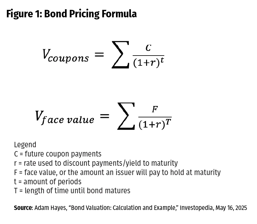
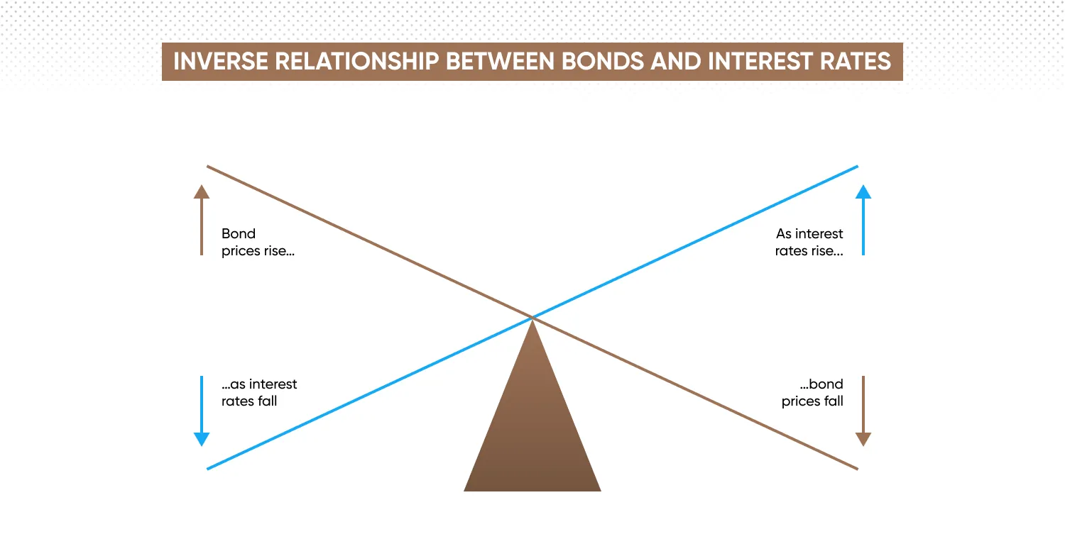
A bond’s quoted price is its clean price, which excludes interest that has accrued since the last coupon payment; the dirty price, what a buyer actually pays at settlement, adds that accrued interest on top. The coupon is the bond’s stated annual interest payment, fixed at issuance as a percentage of face value. Yield to maturity, YTM, is the single discount rate that makes the present value of all remaining coupon payments plus the final principal repayment equal to the bond’s current price, and it is the figure that actually matters, since it reflects the total return an investor earns if the bond is held to maturity, not just the coupon. Current yield, simply the annual coupon divided by the current price, is a cruder measure that ignores the gain or loss built into buying above or below face value, which is why current yield and YTM diverge whenever a bond trades away from par. Yield to call applies to callable bonds, calculating the yield assuming the issuer redeems the bond at the earliest allowable call date rather than holding to final maturity, and yield to worst is simply the lowest of all possible yield outcomes across every call date and final maturity, the appropriately conservative figure to actually use when evaluating a callable bond.

Duration and Convexity

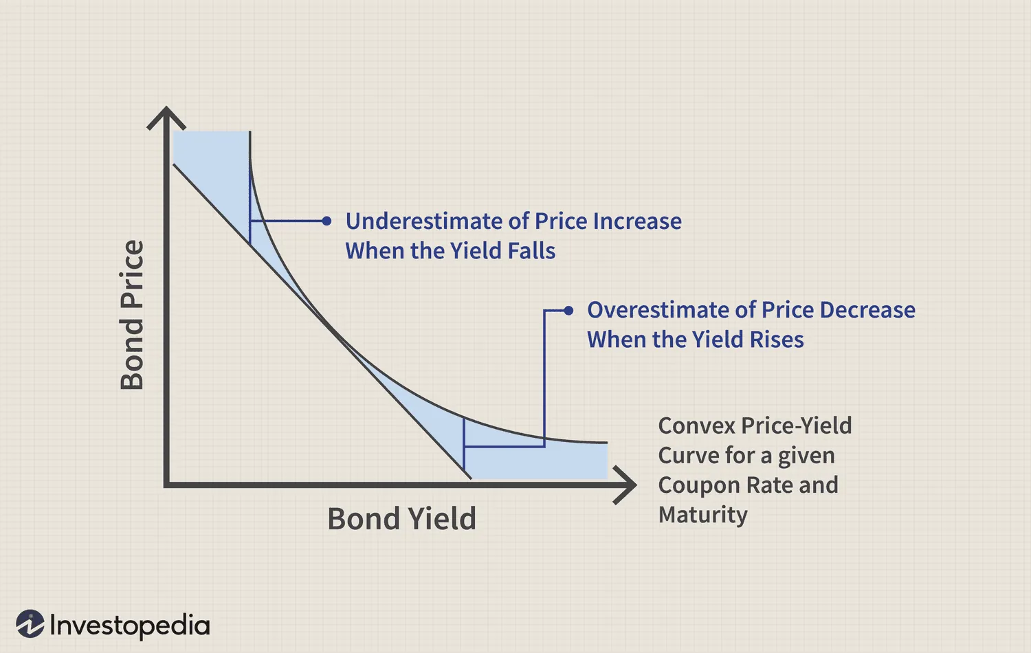
Duration measures a bond’s price sensitivity to a change in interest rates, and the practical rule of thumb is that a bond’s price moves by approximately its duration, in percentage terms, for every one percentage point change in yield: a bond with a duration of seven will fall roughly seven percent in price for a one percentage point rise in rates, and rise roughly the same for a one percentage point fall. Modified duration is this practical, price-sensitivity version; Macaulay duration, the measure it is derived from, is the time-weighted average of when a bond’s cash flows are actually received, expressed in years, and is longer for lower-coupon and longer-maturity bonds, since more of the bond’s value is concentrated further into the future. This relationship is why a thirty-year bond moves far more than a two-year note for the same change in rates, the point already introduced in Part I. Convexity corrects for the fact that duration is only a linear approximation: the true price-yield relationship curves, so duration slightly understates how much a bond’s price rises when yields fall and slightly overstates how much it falls when yields rise, and convexity is the second-order adjustment that captures that curvature, generally a favourable, asymmetric property for the bondholder. Spread duration, or credit duration, measures sensitivity specifically to a change in credit spread rather than the risk-free rate itself, relevant because a corporate bond’s price can move from a change in the market’s perceived credit risk even while government bond yields are unchanged.

The Yield Curve

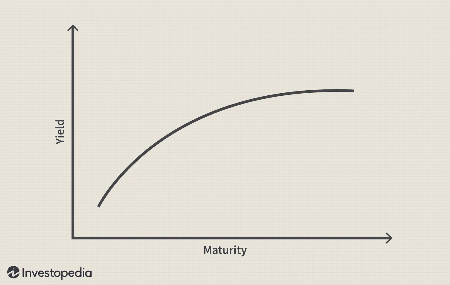
The yield curve plots yield against maturity across otherwise comparable bonds, typically government debt. A normal, upward-sloping curve, where longer maturities yield more than shorter ones, reflects the term premium, the additional compensation investors demand for locking up capital for longer and accepting more uncertainty, and is the shape associated with healthy, expected economic growth. A flat curve suggests the market sees little difference in risk or growth expectations across time horizons. An inverted curve, where short-term yields exceed long-term yields, has historically preceded most recessions in developed markets by several quarters to over a year, though it is a historical tendency rather than a guaranteed signal, and the lag and reliability of that signal has varied considerably across cycles. The curve’s shape also moves in characteristic ways worth naming precisely: a steepening curve sees the gap between short and long yields widen, a flattening curve sees it narrow, and each can happen from either end, a bull steepener (short rates fall faster than long rates, typically an easing central bank), a bear steepener (long rates rise faster, often reflecting rising growth or inflation expectations), a bull flattener (long rates fall faster, often reflecting weakening growth expectations), and a bear flattener (short rates rise faster, typically an aggressively tightening central bank). Reading which of these four is currently happening says something meaningfully different about the macro backdrop than simply noting that “the curve moved.”

Credit Risk in Depth

Credit quality is not a matter of opinion; it is quantified by the major rating agencies, Moody’s, S&P Global, and Fitch, on a scale running from triple-A, the highest quality, down through progressively lower investment-grade tiers to BBB-/Baa3, the line beneath which a bond is reclassified as speculative grade, commonly called high yield or junk. A downgrade below that line can force selling from funds and pension mandates that are contractually restricted to investment-grade holdings only, which is why a rating change often moves a bond’s price more abruptly than the underlying change in default risk alone would suggest. Default risk is the probability an issuer fails to make a scheduled payment; recovery value is what bondholders actually receive if that happens, since a default is rarely a complete loss, senior secured creditors in particular often recover a meaningful portion of face value through the bankruptcy or restructuring process described in Part II. A Credit Default Swap, or CDS, is effectively insurance against an issuer’s default, where the buyer pays a periodic premium in exchange for compensation if a default occurs, and the market-quoted CDS spread is itself watched as a real-time, market-based gauge of perceived credit risk, often reacting faster than a formal ratings action. The Option-Adjusted Spread, OAS, measures the extra yield a bond offers over a comparable government benchmark after adjusting for any embedded options such as a call feature, making it a cleaner apples-to-apples credit-risk comparison than a raw yield spread, and it is the same underlying concept behind the ICE BofA US High Yield OAS covered in Part XII as a market-wide stress gauge. Real yields, the yield remaining after subtracting expected inflation, matter more than nominal yields for judging whether a bond actually compensates an investor after inflation erodes purchasing power; inflation-linked bonds, Treasury Inflation-Protected Securities, TIPS, in the US, have their principal adjusted directly with inflation, explicitly protecting the holder from the erosion nominal bonds are exposed to. Floating-rate bonds pay a coupon that resets periodically against a reference rate rather than staying fixed, which largely insulates their price from the interest-rate-driven moves described above, since the coupon itself adjusts rather than the price needing to. Convertible bonds, introduced in Part II from the issuer’s side, are priced from the investor’s side as a combination of straight bond value plus the value of the embedded option to convert into equity, which is why they tend to behave like a bond when the stock is far below the conversion price and increasingly like the underlying equity as the stock price approaches or exceeds it. Government bonds carry sovereign rather than corporate credit risk, generally lower for developed-market issuers, while emerging market debt carries additional risk layers beyond ordinary corporate credit, currency risk if not dollar-denominated, and political and institutional risk specific to the issuing country, which is why EM debt trades at a meaningfully wider spread than developed-market government debt of comparable duration.

Money Markets

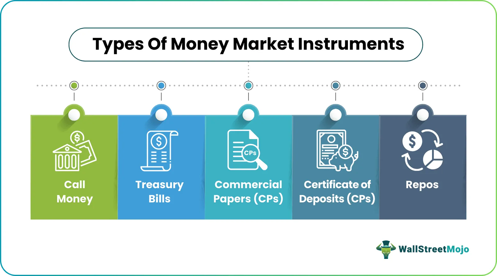
The money market covers debt instruments with maturities under a year, sitting at the short end of the same fixed income universe. Treasury bills are short-dated government debt, typically maturing in a year or less, sold at a discount to face value rather than carrying a stated coupon. Commercial paper is the corporate equivalent, short-term unsecured debt issued by large, creditworthy companies to fund immediate working capital needs. Certificates of deposit are time deposits issued by banks, paying a fixed rate for a fixed term in exchange for the depositor agreeing not to withdraw early without a penalty. Money market funds pool these instruments into a single, highly liquid, low-volatility vehicle, widely used as a cash-equivalent holding. The reference rates underlying this entire market are worth distinguishing clearly: the Fed Funds rate is the US central bank’s own policy target, the rate banks charge each other for overnight loans of reserves; SOFR, the Secured Overnight Financing Rate, has replaced LIBOR as the primary US benchmark for short-term borrowing costs and is based on actual overnight Treasury-repo transactions rather than a survey of estimated rates; €STR serves the equivalent function in the eurozone. OIS, the Overnight Index Swap rate, is a derivative rate based on the expected average overnight rate over a given period and is widely used as a cleaner, lower-credit-risk benchmark for pricing other instruments than a term rate that embeds bank credit risk. The repo market, where institutions borrow cash overnight or short-term against high-quality collateral such as Treasuries, is the plumbing that keeps short-term funding markets liquid and is closely watched by central banks as an early-warning system for system-wide liquidity stress. This entire short-duration universe reprices to track the prevailing policy rate within days of a central bank decision, since duration close to zero means there is essentially no price sensitivity standing between the instrument and the new policy rate, which is why money market yields are the fastest and most direct real-time read on where short-term rates actually stand.

Part VII: Derivatives and Structured Products

Options: The Building Blocks

A call option gives the buyer the right, not the obligation, to purchase the underlying asset at a fixed strike price on or before expiration; a put option gives the right to sell. Moneyness describes the relationship between the strike and the current underlying price: a call is in-the-money (ITM) when the underlying trades above the strike, at-the-money (ATM) when it sits at the strike, and out-of-the-money (OTM) when the underlying trades below it, with puts working in the mirrored direction. An option’s premium splits into two components: intrinsic value, the amount by which it is currently ITM, zero for any ATM or OTM option, and extrinsic value, everything else in the premium, driven by time remaining and implied volatility, which is exactly the component that decays to zero by expiration regardless of what the underlying does. Exercise is the buyer choosing to actually use their right to buy or sell at the strike; assignment is what happens to the seller of that option when the buyer exercises, obligating the seller to fulfil the trade, which is why selling an option, as opposed to buying one, carries the risk of an obligation rather than merely a right. American-style options can be exercised at any point up to expiration; European-style options can only be exercised at expiration itself, a distinction that mainly affects early-exercise risk for the seller and is set by the contract specification rather than by choice.

Put-Call Parity

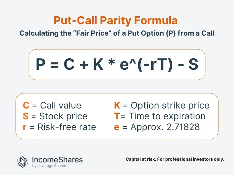
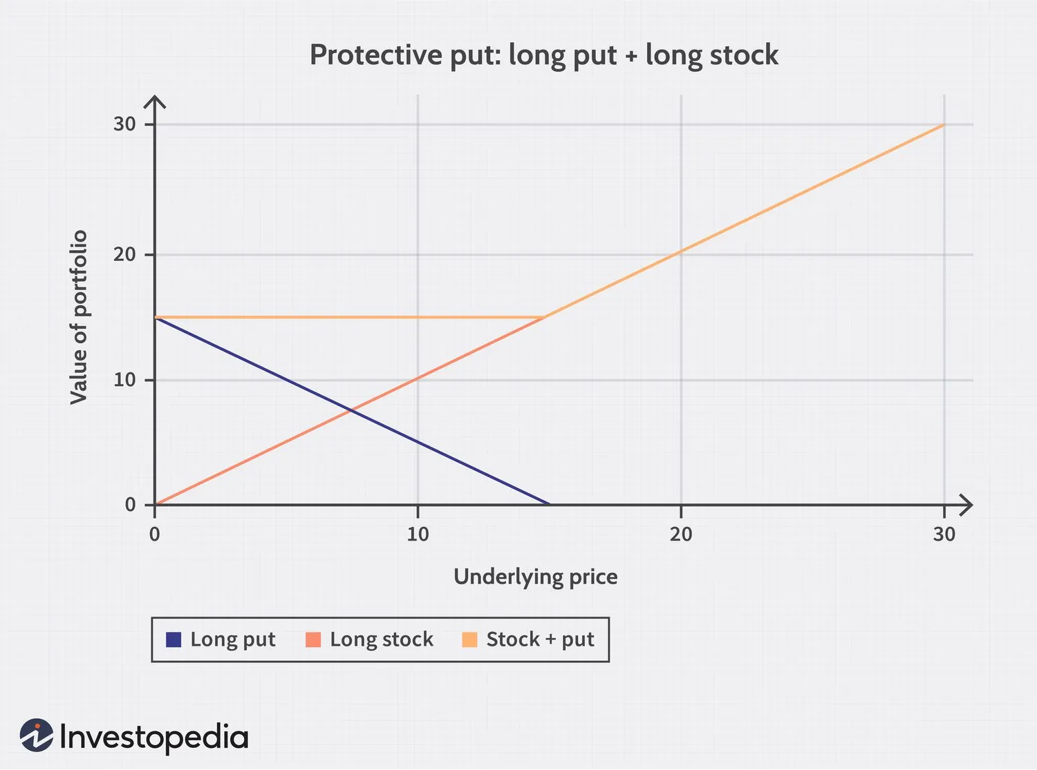
A call and a put sharing the same strike and expiry are not independent prices; they are mathematically linked to each other and to the underlying through a no-arbitrage relationship called put-call parity. In plain terms, buying a call and selling a put at the same strike and expiry produces the same payoff as simply owning the underlying asset outright, financed at the risk-free rate, which means the call price minus the put price must equal the underlying price minus the present value of the strike. If that relationship is ever violated by more than transaction costs allow, an arbitrageur can construct a combination of the option, its counterpart, and the underlying that locks in a riskless profit, which is exactly the mechanism that keeps the relationship holding in practice across liquid option markets. Put-call parity is less a trading signal in its own right and more the structural glue tying every other concept in this Part together: it is why a protective put and a covered call are, economically, simply different packagings of the same underlying exposure.

Implied Volatility and the Volatility Surface

Implied volatility, IV, is the market’s forward-looking estimate of how volatile the underlying will be, backed out of the option’s current price, and is the single biggest driver of extrinsic value; historical (or realised) volatility, by contrast, measures how volatile the underlying has actually been over some recent past period, and the gap between the two is itself a piece of information, since options frequently price in more (or less) future movement than recent history alone would suggest. IV is not uniform across every strike and expiration for the same underlying. The volatility smile describes IV rising for both far ITM and far OTM strikes relative to ATM strikes; the volatility skew, more commonly observed in equity index options, describes OTM puts carrying persistently higher IV than OTM calls, reflecting sustained demand for downside protection. The term structure of volatility describes how IV varies across different expiration dates for the same underlying, and it typically steepens sharply around a known event such as the earnings date covered in Part II, precisely the mechanism behind the volatility crush already introduced there. IV rank and IV percentile both contextualise a stock’s current IV level against its own history over a lookback period, generally a year, and are widely used to judge whether option premium is currently rich or cheap relative to that stock’s own normal range, information a raw IV number alone does not provide.

The Greeks

The Greeks quantify exactly how an option’s price responds to changes in the variables that determine it, and are the practical tool for understanding an option position’s actual risk beyond simple directional exposure.

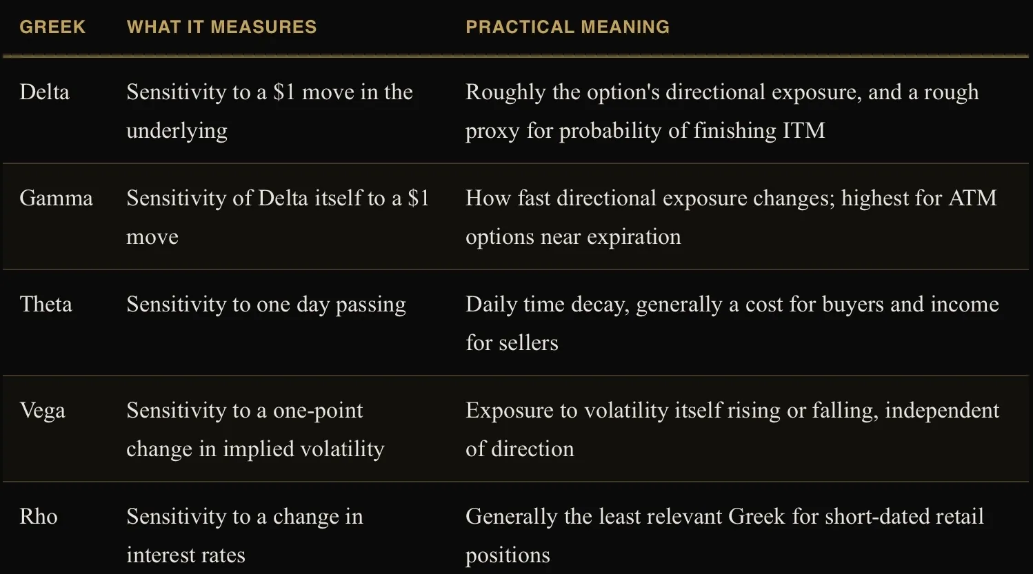
Zero-Days-to-Expiration options, commonly called 0DTE, expiring the same day they are traded, have grown into a substantial share of total options volume in major index products, and they represent Theta and Gamma taken to their most extreme: time decay accelerates dramatically in an option’s final hours, and Gamma, the rate of change of Delta, becomes correspondingly unstable, meaning a 0DTE position’s directional exposure can shift sharply within minutes as the underlying moves. They are used by some traders for short-term income generation and by others for pure, low-cost directional speculation, and the same volatility crush dynamic introduced in Part II applies within a single trading session rather than across days, making 0DTE positions considerably less forgiving of poor timing than longer-dated options.

Options Strategies

Every options strategy is a specific combination of long or short calls and puts built to express a defined view on direction, volatility, or both, with a defined maximum profit and maximum loss.

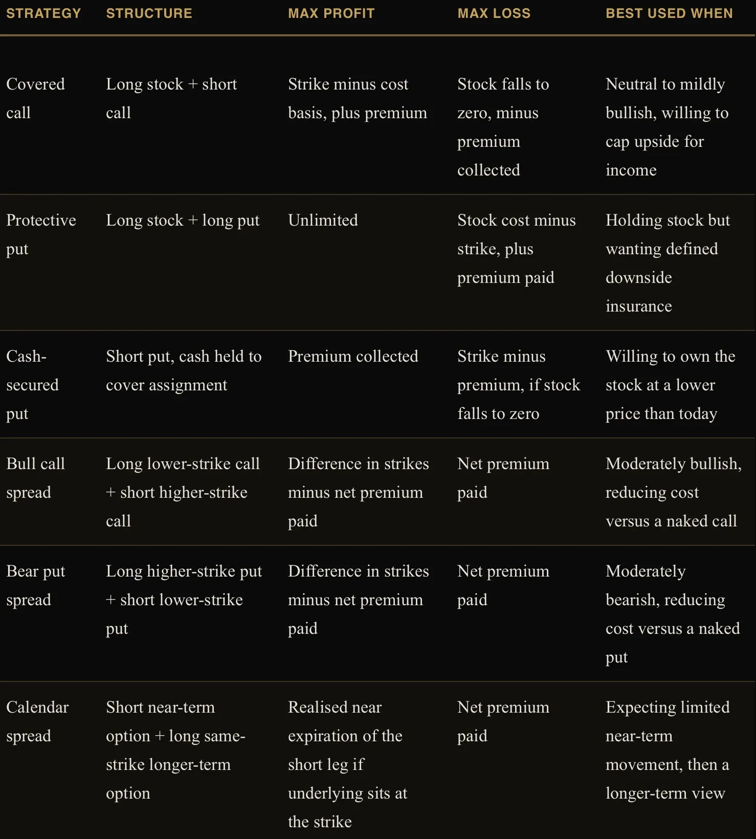
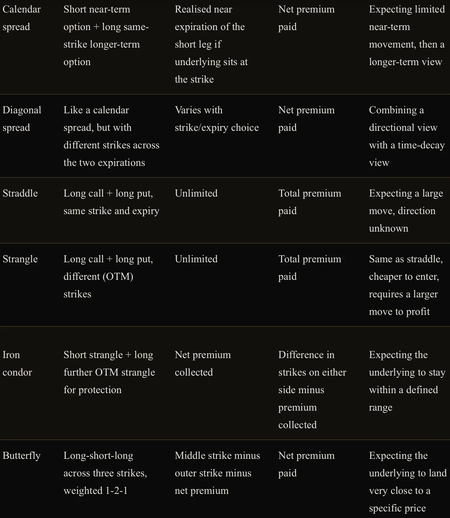
Every strategy above carries a directional exposure (bullish, bearish, or neutral), a volatility exposure (long volatility strategies like straddles benefit from IV rising; short volatility strategies like iron condors benefit from IV falling or staying flat), a time-decay profile (net option buyers lose to Theta, net option sellers collect it), and, for any position involving a short option, assignment risk, the possibility of being assigned the underlying position before expiration, which is generally most relevant just before a dividend’s ex-date for short calls, tying back to the dividend mechanics in Part II.

Futures and Forwards

A futures contract specifies an exact contract size (the quantity of the underlying per contract), a tick size (the smallest allowable price increment) and corresponding tick value (the dollar value of that smallest increment), which together determine the actual dollar profit or loss per point of price movement. Futures are margined rather than paid for in full: initial margin is the deposit required to open a position, a small fraction of the contract’s full notional value, which is the source of the leverage described in Part IV, and maintenance margin is the minimum account balance that must be sustained afterward, with a margin call issued if the account falls below it. Futures positions are marked-to-market daily, meaning gains and losses are settled in cash to the account every single day rather than only upon closing the position, which is a meaningfully different cash-flow experience than holding an option or a stock. Settlement at expiration is either physical (actual delivery of the underlying commodity or asset) or cash-settled (a final cash payment reflecting the difference), with the large majority of retail-accessible futures on financial underlyings settling in cash. A forward contract is a futures contract’s OTC cousin: the same basic agreement to buy or sell an asset at a set price on a future date, but individually negotiated between two parties rather than standardised and exchange-traded. Because a forward is not cleared through the clearing-house mechanism covered in Part III, it carries direct bilateral counterparty risk that an exchange-traded future does not, and it is not marked-to-market daily, meaning gains and losses accrue silently until the contract’s actual settlement date rather than being settled in cash along the way.

The futures curve, the set of prices for the same underlying across different expiration months, can slope in either direction: contango describes futures prices above the current spot price, typically reflecting storage and financing costs for physical commodities; backwardation describes futures prices below spot, often reflecting near-term supply tightness or high current demand for immediate delivery. The theoretical driver behind this shape has a name: cost of carry, the financing cost of holding the underlying until delivery, plus any storage cost, minus any income the asset generates in the meantime, a dividend or the convenience yield introduced in Part XV. A positive net cost of carry pushes the futures price above spot into contango; a negative one, income exceeding financing and storage cost, pushes it into backwardation, formalising the mechanism behind both financial and commodity futures curves in a single framework. The basis is simply the gap between the futures price and the spot price at any given moment, and it converges to zero as expiration approaches. Roll yield is the return, positive or negative, earned specifically from rolling an expiring futures contract into the next one, positive in backwardation (selling the expiring contract at a relatively higher price and buying the next one cheaper) and negative in contango, which is precisely why a commodity ETC’s realised return over time can diverge meaningfully from the simple change in the spot price, a point revisited directly in Part XV. This is also why a futures-based instrument’s total return has several distinct components worth naming separately: the spot return (the change in the underlying’s own price), the futures return (spot return plus or minus roll yield), the collateral return (interest earned on the margin capital backing the position, since only a fraction of notional value is actually posted), and total return (the sum of all of the above), which is the figure that actually determines what an investor holding a futures-linked product experiences.

Swaps

A swap is an agreement between two parties to exchange one stream of cash flows for another, and the swap market is where the large majority of institutional interest-rate and currency risk is actually managed, well beyond what appears in the exchange-traded and retail-accessible instruments covered elsewhere in this guide. An interest rate swap exchanges a fixed interest rate for a floating one, calculated against the same notional amount, without any exchange of principal; a company with floating-rate debt worried about rising rates can swap into a fixed rate, or a fund with a specific view on rates can take either side purely for exposure, without ever touching the underlying loan itself. An FX swap combines a spot currency transaction with an offsetting forward transaction in the opposite direction, functioning as the core plumbing of institutional cross-currency funding: it lets an institution temporarily convert one currency into another and back again at a rate reflecting the interest-rate differential between the two, the same carry-trade economics introduced in Part XIV, expressed as a single packaged instrument. A Total Return Swap exchanges the total return, price appreciation plus any income, of a reference asset for a financing rate, letting one party gain full economic exposure to an asset without ever owning it directly, precisely the mechanism behind the synthetic ETF replication already covered in Part VIII, and a common tool for institutions seeking leveraged or offshore exposure without the operational complexity of holding the underlying asset itself.

Structured Products for European Retail Investors

Warrants are bank-issued instruments economically similar to a listed option, a call or put on an underlying with a strike and expiry, but issued and priced by a bank rather than traded on a standardised options exchange. A knock-out certificate embeds a barrier: the product is automatically terminated, typically at or near zero value, the instant the underlying touches that barrier, regardless of any subsequent recovery, and because the barrier sits close to the current price, the effective leverage of a knock-out certificate changes constantly as price moves toward or away from it. A factor certificate instead targets a fixed daily leverage multiple, resetting each day, which produces the same volatility-decay behaviour explained in full for leveraged ETFs in Part VIII: its multi-day return can diverge substantially from the simple leverage multiple applied to the underlying’s multi-day return. A discount certificate is purchased below the underlying’s current price in exchange for a capped maximum payout, suited to a moderately bullish or neutral view with a defined ceiling. A bonus certificate pays a defined bonus level at maturity provided the underlying never touches a lower barrier during the product’s life, and otherwise simply tracks the underlying, effectively a conditional buffer against moderate declines. A reverse convertible pays an enhanced coupon in exchange for the investor bearing the downside risk of the underlying below a defined level, economically similar to having sold a put option in exchange for income. ETCs (Exchange-Traded Commodities), ETNs (Exchange-Traded Notes), and the broader ETP (Exchange-Traded Product) category built around them are unsecured debt obligations of the issuer that track an underlying index or commodity, distinct from an ETF’s fund structure covered in Part VIII, and a tracker certificate is a simple, undated version of the same basic idea, generally following an index one-to-one before costs.

The risk vocabulary specific to this entire category is worth stating explicitly, since it is exactly what gets glossed over in retail marketing. Issuer risk is the single most important one: a certificate or warrant is unsecured debt issued by the bank, not fund ownership of the underlying assets, meaning the investor bears the issuer’s own credit risk on top of the underlying’s market risk, a structural difference from an ETF that most retail marketing materials do not emphasise. Counterparty risk is the closely related exposure to the specific bank or dealer standing behind the product’s pricing and eventual payout. Barrier risk and knock-out risk describe the risk of the underlying touching a defined level and either permanently terminating the position (knock-out) or altering the payout structure (barrier products generally). Financing costs are embedded directly in the spread between a leveraged product’s market price and its theoretical value, meaning two products advertising identical stated leverage can carry a different effective cost of carry, and that spread, along with general liquidity risk (how easily the specific product can be sold before maturity without a punitive price concession) and currency risk (if the underlying and the product are denominated in different currencies), and tracking error (deviation from the stated underlying’s actual performance) together determine the true cost of holding the product, well beyond the headline leverage figure alone.

Part VIII: ETFs

Exchange-Traded Funds have become the default building block of retail portfolios over the past two decades, and for good structural reasons. But an ETF is not automatically a safe or a simple product, and treating every ETF as interchangeable with a broad index fund is a mistake worth correcting directly.

What Actually Happens When an Investor Buys an ETF

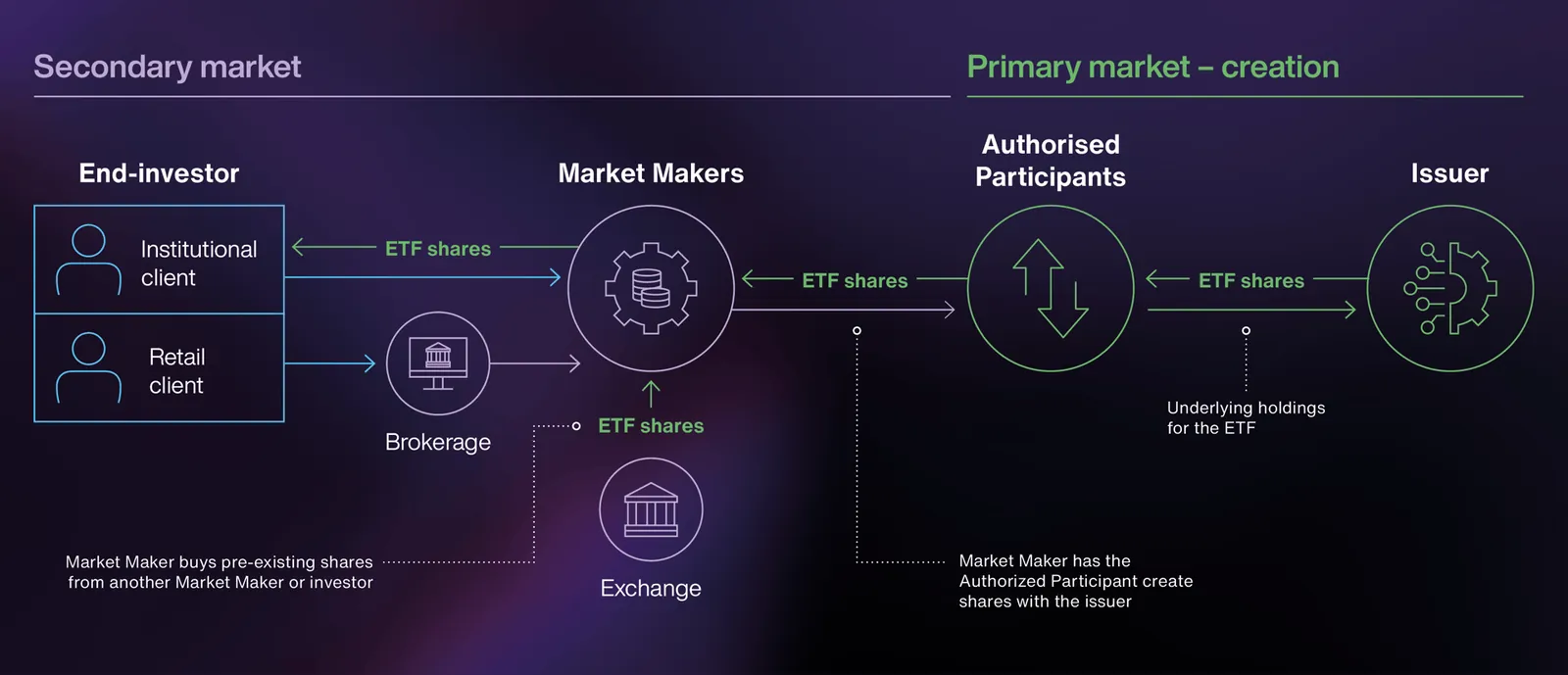
An ETF is a fund, legally distinct from the bank-issued debt structures covered in Part VII, that holds a basket of underlying assets and issues shares against that basket, and its mechanics are worth understanding precisely because most of an ETF’s genuine risks live inside them rather than in the headline strategy. Physical replication means the fund actually buys and holds the underlying securities, either through full replication (every constituent, at its index weight) or sampling (a representative subset that closely tracks the index without holding every single name, common for very broad or illiquid indices). Synthetic replication instead holds a different collateral basket and enters into a swap agreement with a bank counterparty, who contractually delivers the index’s return in exchange for a fee, which introduces counterparty risk to that swap provider on top of ordinary market risk, a distinction worth checking in an ETF’s documentation rather than assuming. Even fully “physical” ETFs commonly engage in securities lending, lending out their underlying holdings to short sellers, the same mechanism described for individual shares in Part III, in exchange for extra revenue that modestly improves the fund’s return, but this too introduces counterparty risk to whoever is borrowing the securities, generally mitigated by requiring posted collateral but not eliminated entirely.

The mechanism that keeps an ETF’s market price closely tethered to the value of its underlying holdings is the creation and redemption process, carried out exclusively by Authorised Participants, large institutional trading firms who can exchange a basket of the underlying securities for new ETF shares (creation) or ETF shares for the underlying basket (redemption), directly with the fund. Whenever the ETF’s market price drifts meaningfully away from its Net Asset Value, NAV, the per-share value of the actual underlying holdings, this arbitrage mechanism gives Authorised Participants a direct profit incentive to trade against that gap, which is what keeps a healthy ETF’s premium or discount to NAV small under normal conditions, though that gap can widen meaningfully during periods of market stress or for ETFs holding genuinely illiquid underlying assets.

Costs and Structure

Tracking difference measures the actual gap between an ETF’s total return and its benchmark index’s total return over a period, capturing the sum of all costs and frictions; tracking error measures the volatility, the consistency, of that gap over time, and a fund can have a small average tracking difference but a large, erratic tracking error, which is itself a signal of a less well-managed product. The Total Expense Ratio, TER, is the fund’s stated annual management cost, but it is not the only cost an investor bears: the bid-ask spread paid on every purchase and sale, and any transaction costs the fund itself incurs rebalancing its holdings, both add to the real, all-in cost of ownership beyond the TER alone. Assets Under Management, AUM, is a rough proxy for a fund’s viability and liquidity, since a very small or shrinking ETF carries meaningfully elevated fund-closure risk, the fund being liquidated and its holdings forcibly sold, an inconvenient and potentially tax-inefficient event for holders. Accumulating share classes reinvest dividends and income internally rather than distributing cash, growing NAV directly, while distributing share classes pay income out to holders as cash, a distinction that matters both for cash-flow needs and for the tax treatment covered in Part XVIII. Fund domicile, the legal jurisdiction the fund itself is registered in, and UCITS, the regulatory framework the large majority of European-listed ETFs operate under, together determine what investor protections and reporting standards apply and are worth checking rather than assuming are identical across every product marketed to a European investor. Currency hedging, available as a separate share class on many international ETFs, removes the currency-translation effect described in Part XIV from the fund’s return, at the cost of an additional, ongoing hedging expense.

Index Methodology and Concentration

An ETF is only ever as sound as the index it tracks, and index methodology, how constituents are selected and weighted, and index rebalancing, how often and by what rule that weighting is periodically updated, directly determine what an investor actually owns and how it changes over time, tying back to the mechanical rebalancing flows described in Part II. Market-cap weighting, the standard default for most broad index ETFs, allocates more weight to larger companies, which means a cap-weighted fund’s return becomes increasingly concentrated in its largest constituents as they grow, a dynamic already flagged as a systemic consideration in this guide’s original ETF discussion. Equal weighting instead allocates identical weight to every constituent regardless of size, reducing concentration but increasing the practical cost of the more frequent rebalancing required to maintain those equal weights. Concentration risk applies just as directly to thematic and sector ETFs, which can hold a genuinely small number of underlying names despite carrying the word “fund” in their description, offering far less true diversification than a broad index product.

The Risks That Get Glossed Over

Leveraged and inverse ETFs, which aim to deliver a multiple or the inverse of an index’s daily return, suffer from volatility decay for the same structural reason described for factor certificates in Part VII: because they reset their leverage every single day, their return over any period longer than a day or two can diverge substantially, and sometimes catastrophically, from the simple multiple of the underlying index’s return over that same period, even when the underlying index has ended up roughly flat. Niche and illiquid ETFs, commodity ETFs and ETCs among them, can carry a wide bid-ask spread and real tracking error against their stated benchmark, and in a genuine liquidity crisis, the ETF wrapper’s promise of continuous tradability can strain against the underlying market’s actual ability to transact, particularly in fixed income and less liquid asset classes.

The honest conclusion is that ETFs are an excellent tool and a poor blanket assumption. The specific ETF, its replication method, its underlying liquidity, its index methodology, and its all-in cost all matter as much as the decision to use an ETF wrapper in the first place.

Part IX: Trading and Investment Strategies

Market Efficiency and Why Strategies Exist At All

Every strategy in this Part implicitly claims that markets are not perfectly efficient, that some edge exists to be found through fundamental research, technical structure, or behavioural patterns, so it is worth briefly stating the theory that argues otherwise. The Efficient Market Hypothesis holds that asset prices already reflect available information, and comes in three commonly cited forms: weak form, where prices reflect all past price and volume data, meaning technical analysis alone offers no durable edge; semi-strong form, where prices reflect all publicly available information, meaning fundamental analysis of public filings offers no durable edge either; and strong form, where prices reflect even private, non-public information, under which no legal method of analysis offers a durable edge at all. In its strict form, EMH sits uneasily alongside the persistent, well-documented anomalies covered throughout this guide, momentum, value, size, and the post-earnings announcement drift described in Part II among them, as well as calendar effects, statistically recurring seasonal patterns such as unusually strong average returns around the turn of the month or the turn of the year, that have shown up with some consistency across long historical samples despite no obvious fundamental reason for a calendar date itself to matter. The practical, working position most professional research operates from sits between the extremes: markets are efficient enough, most of the time, that a genuine and durable edge is hard to find and harder to sustain, but not so perfectly efficient that structure, discipline, and a genuine informational or analytical edge cannot produce a real one, which is the working assumption behind every strategy and every framework the rest of this guide is built on.

Every strategy is an answer to a specific question: over what time horizon, and based on what kind of edge, is this position expected to make money. Confusing strategies, or running several at once without knowing which one is actually in control of a given position, is one of the most common sources of retail losses.

Buy and Hold

The simplest strategy in existence: acquire quality assets and hold them through volatility on the belief that, over sufficiently long periods, markets and quality businesses compound upward. Its main requirement is not analytical skill but psychological discipline through drawdowns.

Dollar-Cost Averaging

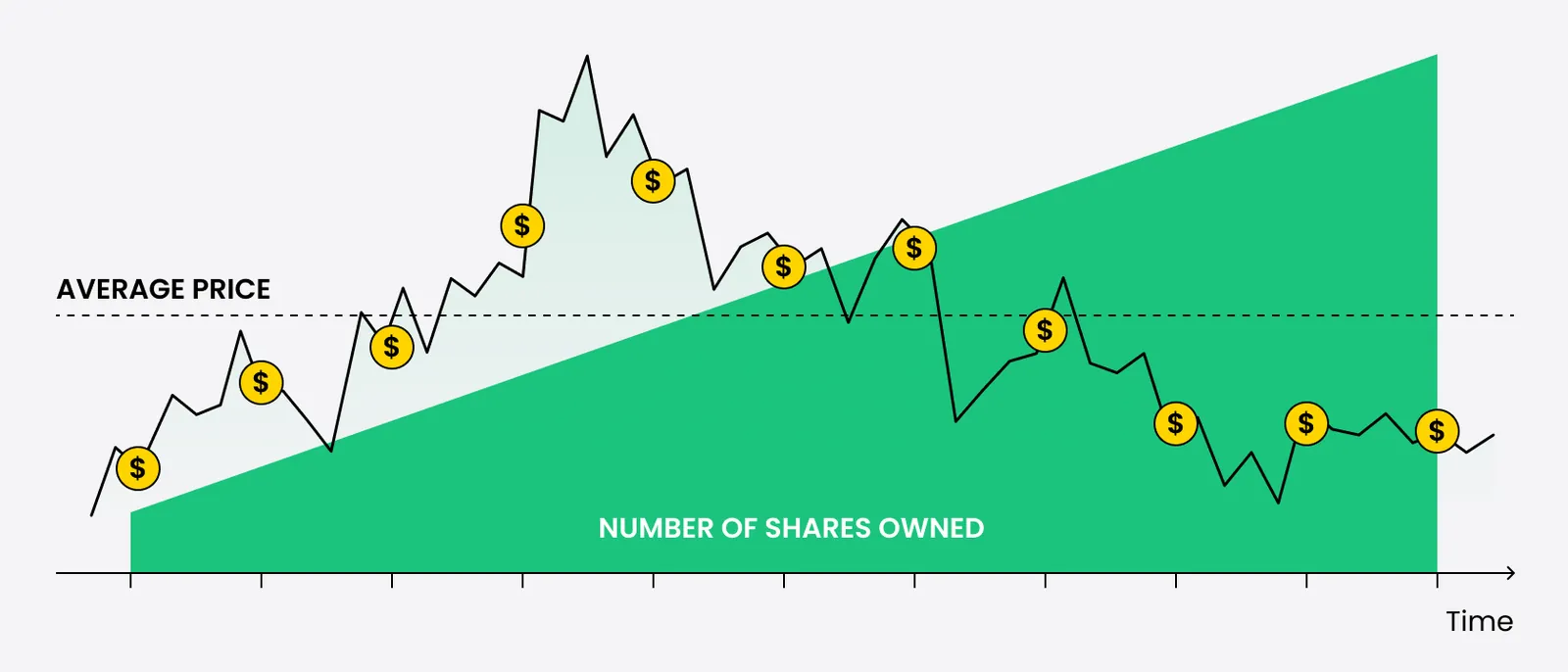
Investing a fixed amount at regular intervals regardless of price. This removes the need to time entries and smooths the average purchase price over time, at the cost of sometimes buying into strength that a more tactical investor would have avoided.

Value Investing

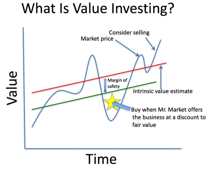
Identifying companies trading below their estimated intrinsic worth, typically based on depressed valuation multiples relative to earnings, assets, or cash flow, and holding until the market closes that gap. It requires patience, since undervaluation can persist or worsen for extended periods before it resolves, and it requires the valuation discipline covered in full in Part V to distinguish a genuinely mispriced business from one that is cheap for good reason.

Growth Investing

Prioritising companies with above-average revenue and earnings growth, often at premium valuations, on the view that the growth trajectory itself justifies the multiple being paid today. The primary risk is a derating: even a company that keeps growing can see its share price fall hard if growth decelerates relative to what was priced in, the multiple-contraction dynamic covered in Part V.

Momentum Investing

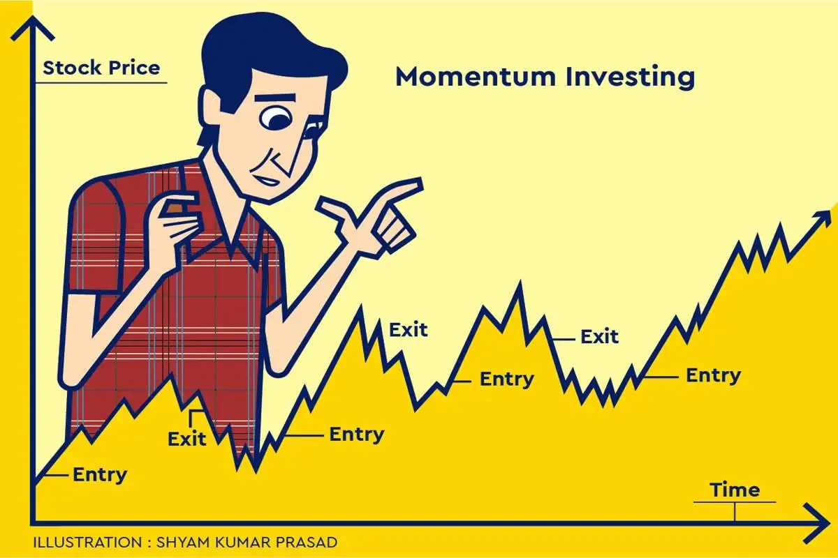
Buying assets that have recently outperformed on the empirically well-documented tendency for strong recent performance to persist over intermediate horizons, and selling or shorting recent laggards. Momentum works until it reverses sharply, which is why disciplined position sizing matters more here than in almost any other style.

Trend Following

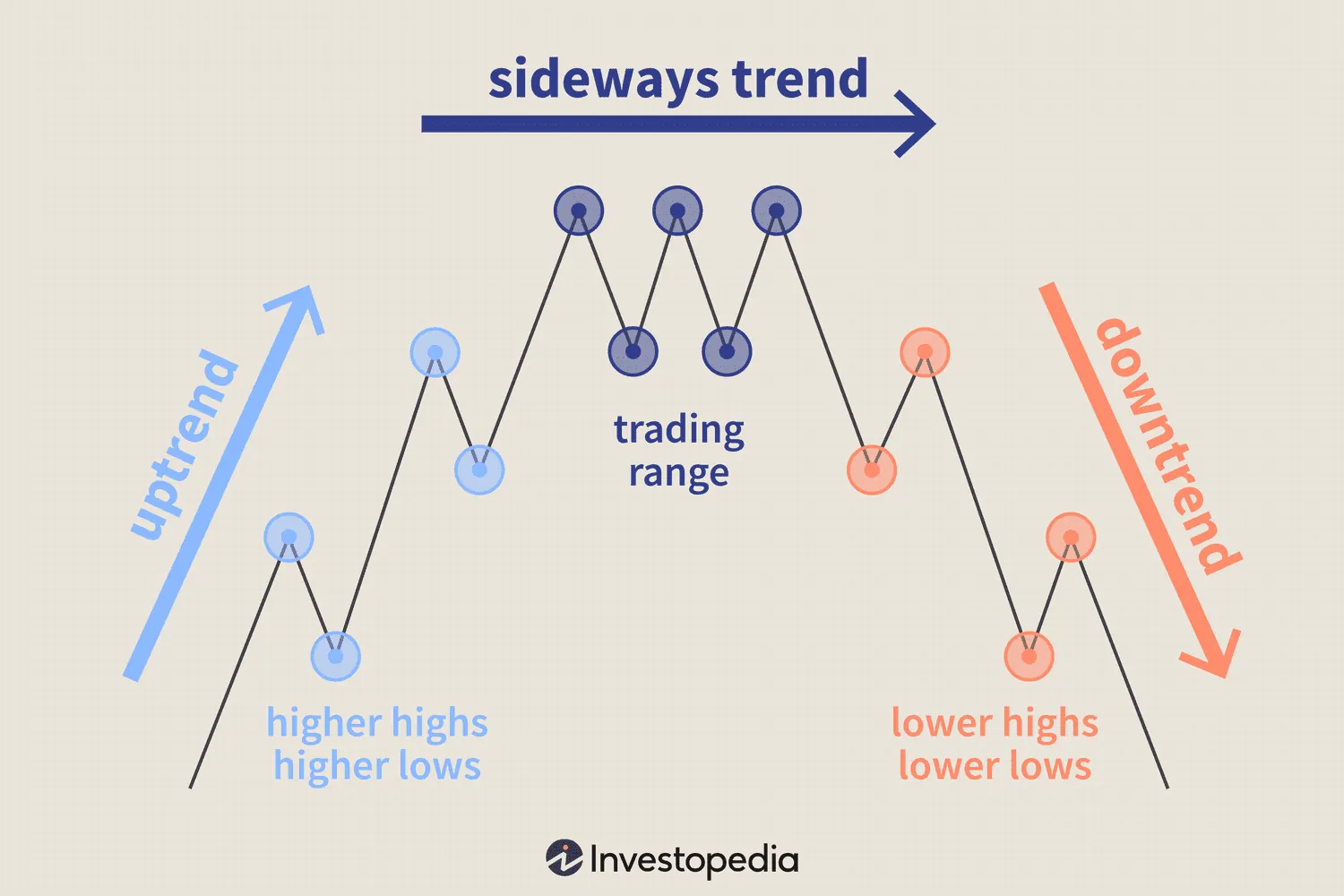
A systematic approach that stays with an established directional move across any asset class, using moving averages, breakouts, or structural price levels to define what “trend” means, and exits when that trend structurally breaks. It underperforms in sideways, choppy markets and performs best during sustained directional regimes, the regime-dependency covered directly in Part XIII.

Mean Reversion

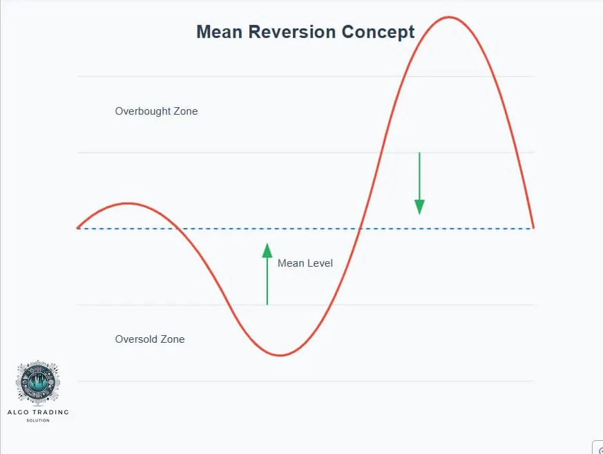
The opposite logic to momentum: prices that have moved unusually far from a statistical or technical baseline tend to snap back toward it. Mean reversion strategies typically operate on shorter time horizons and require strict risk control, because a genuine regime change can look identical to a temporary overextension until it is too late.

Swing Trading

Holding positions for several days to several weeks to capture a defined price swing within a larger trend, blending elements of technical timing with a moderate holding period. It sits between the patience of investing and the speed of day trading.

Day Trading

Opening and closing positions within a single session, with no overnight exposure. It demands constant attention, low transaction costs, and a statistical edge repeated across a very high number of trades, and it is, by a wide margin, the hardest of these approaches to execute profitably on a sustained basis.

Elliott Wave and Structural Technical Analysis

A method that interprets price action as a sequence of impulsive and corrective wave structures, governed by Fibonacci-derived proportional relationships between waves. Rather than predicting a single price target, it defines a structural framework of probable zones and, critically, a clear invalidation level at which the interpretation is proven wrong.

More about Elliott Waves:

Elliott Wave Framework

Options Income Strategies

Selling covered calls against an existing holding, or cash-secured puts against a desired entry price, to generate income from option premium. These strategies exchange unlimited upside, or an immediate cash outlay, for a defined and often steady income stream, and are covered mechanically in full in Part VII.

Pairs Trading and Market-Neutral Strategies

Simultaneously taking a long position in one asset and a short position in a correlated one, profiting from the relative movement between the two rather than the direction of the broader market. This isolates a specific thesis, such as one company outperforming a sector peer, while hedging out much of the general market risk.

No strategy is universally correct. Each is a tool suited to a specific time horizon, a specific type of market behaviour, and a specific investor temperament, and the strategy has to be chosen to fit the investor, not the other way around.

Part X: The Technical Analysis Toolkit

Professional desks do not watch hundreds of indicators. They watch a relatively small, well-chosen set that captures structure, momentum, and volatility, and they read those tools together rather than in isolation. What follows is organised by what each category is actually trying to answer, not as an undifferentiated list.

Reading Price Structure Directly

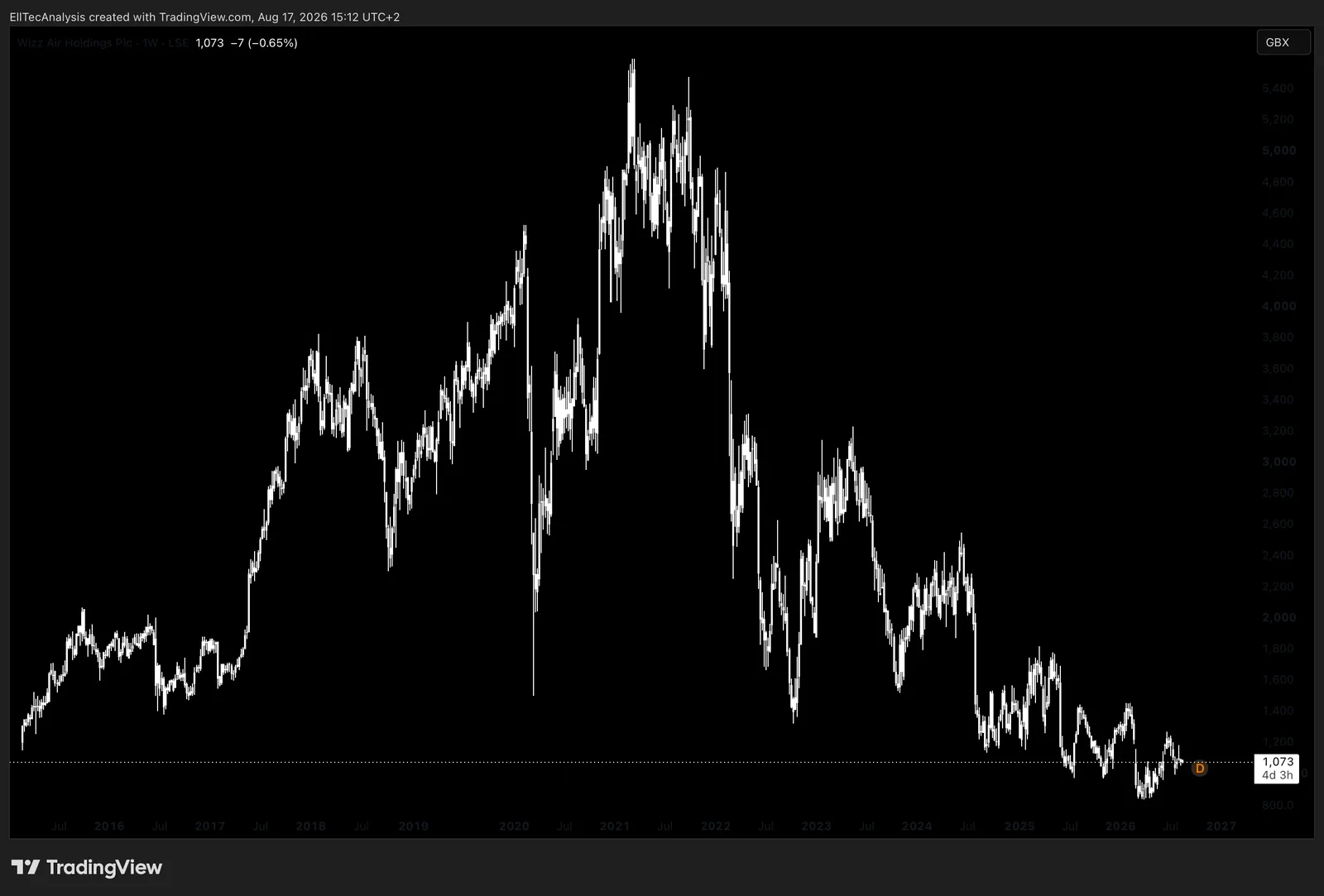
The most basic and, in practice, one of the most reliable reads of trend comes before any indicator is applied at all: a sequence of higher highs and higher lows defines an uptrend; a sequence of lower highs and lower lows defines a downtrend, and the first sign of trend change is often simply the sequence breaking. Support and resistance are price levels where buying or selling pressure has previously been strong enough to reverse or stall a move, and they frequently coincide with the high-volume nodes described in the Volume and Fixed Range Volume Profile discussion below, since a price level many participants previously transacted at is exactly where many of them have an incentive to defend a position now. Trendlines and channels connect a series of swing highs or lows to visualise the current structure, genuinely useful for framing a move, but they are inherently subjective and redrawable after the fact, which is why they work best as a supporting visual rather than a standalone trading signal. A breakout is price moving decisively beyond a defined structural level; a false breakout is the same move failing and reversing back inside the prior range shortly after, often the result of the stop-hunting dynamic already described around liquidity heatmaps, which is why breakout traders generally wait for a confirming close beyond the level rather than acting on the first touch. A gap is price opening away from the prior session’s close, and not all gaps carry equal information: a common gap on light volume is usually just noise, a breakaway gap on heavy volume at the start of a new structural move tends to mark genuine participation, and an exhaustion gap appearing after an extended move often marks its final, climactic stage rather than its continuation. Candlestick patterns, a small handful of genuinely useful ones such as an engulfing candle or a long-wicked reversal candle at a known structural level, add texture to this picture, but they carry far more weight when they appear at a level already identified as significant by other means than they do in isolation.

Moving Averages, VWAP, and Trend Tools

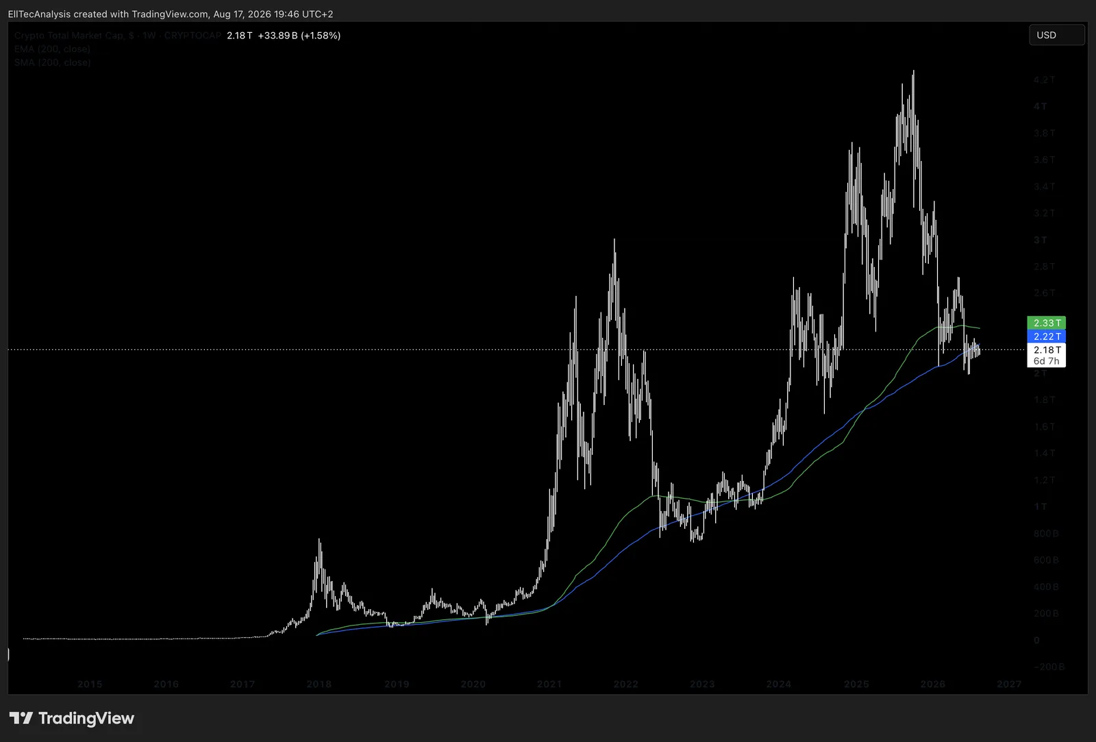
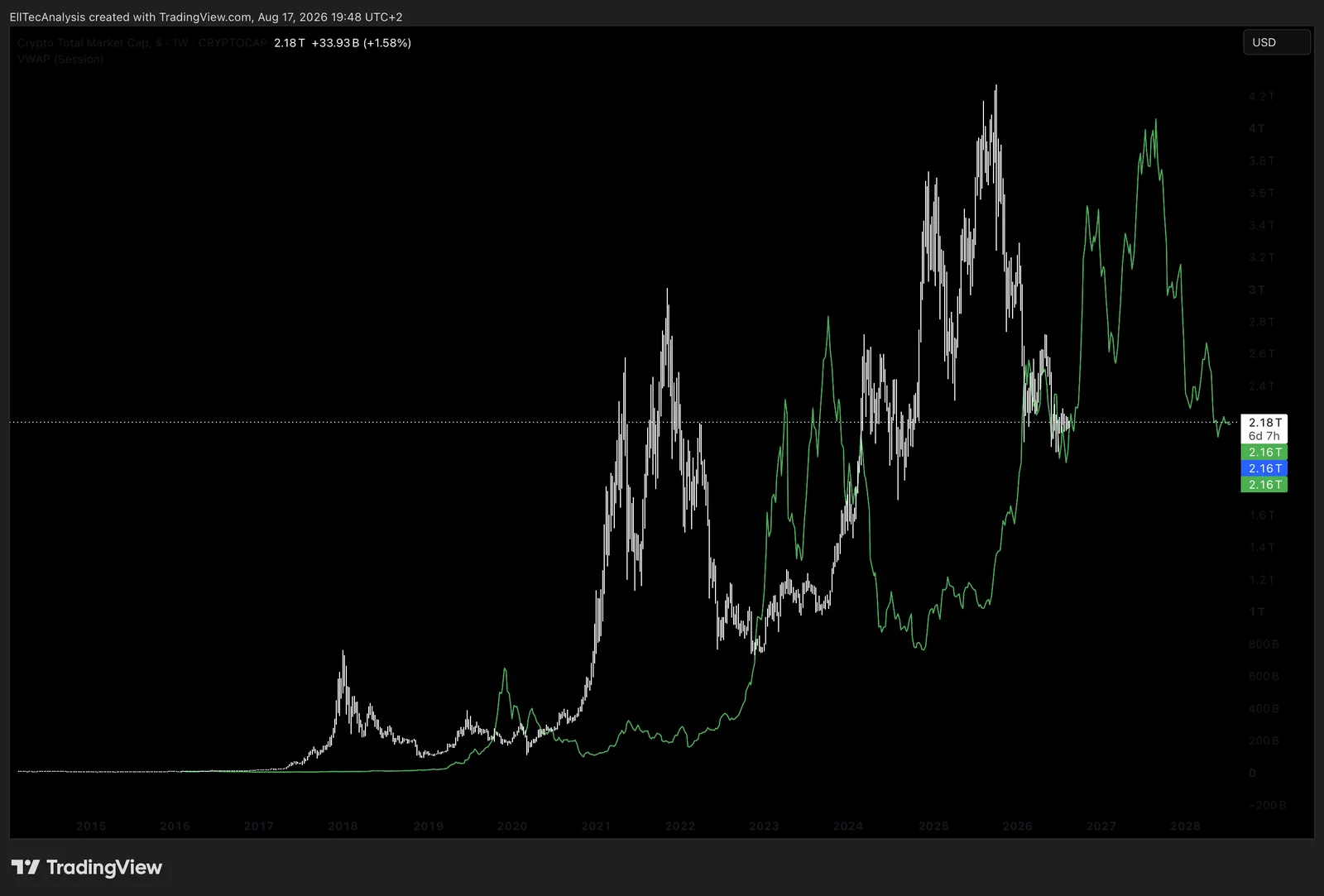
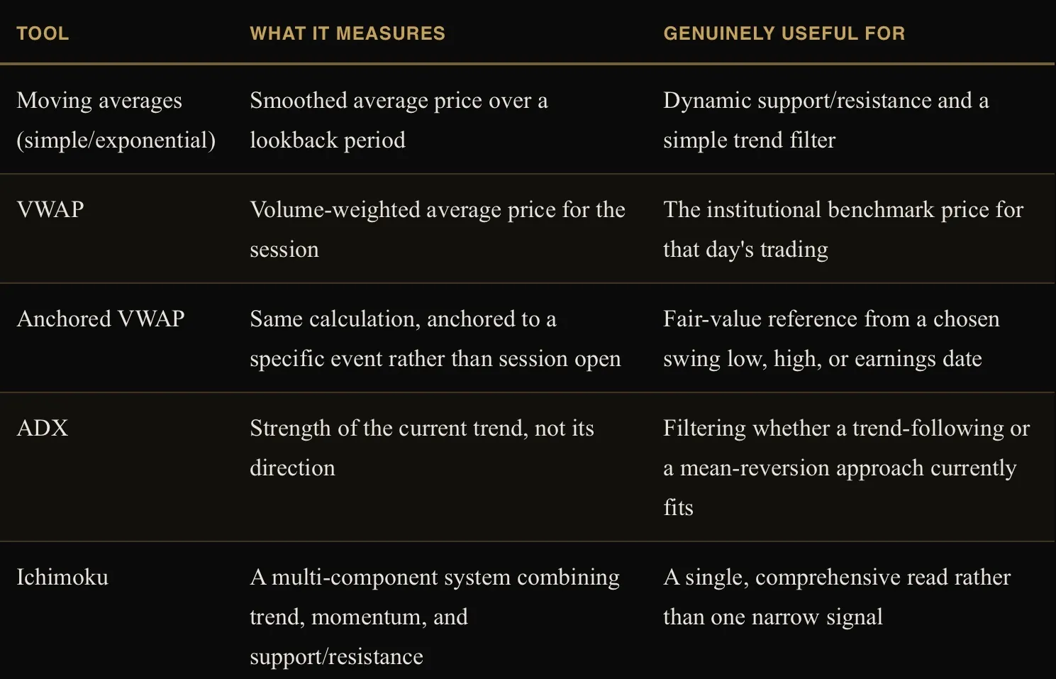
Oscillators, Volume Confirmation, and Volatility

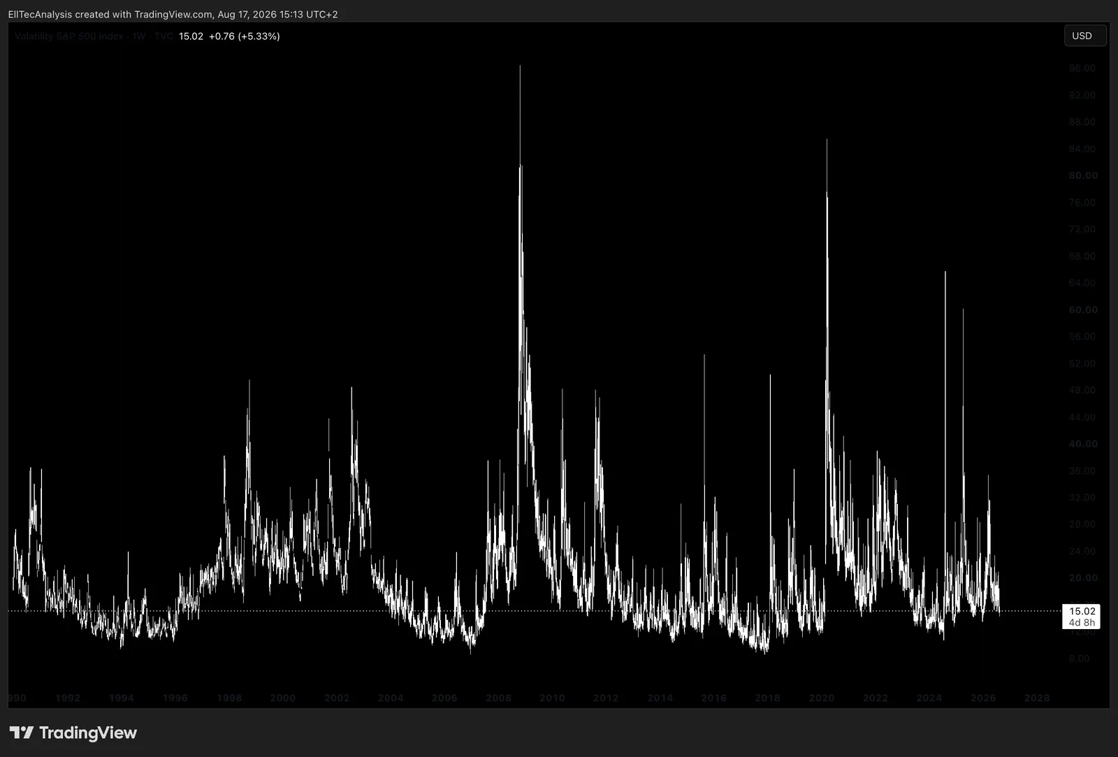
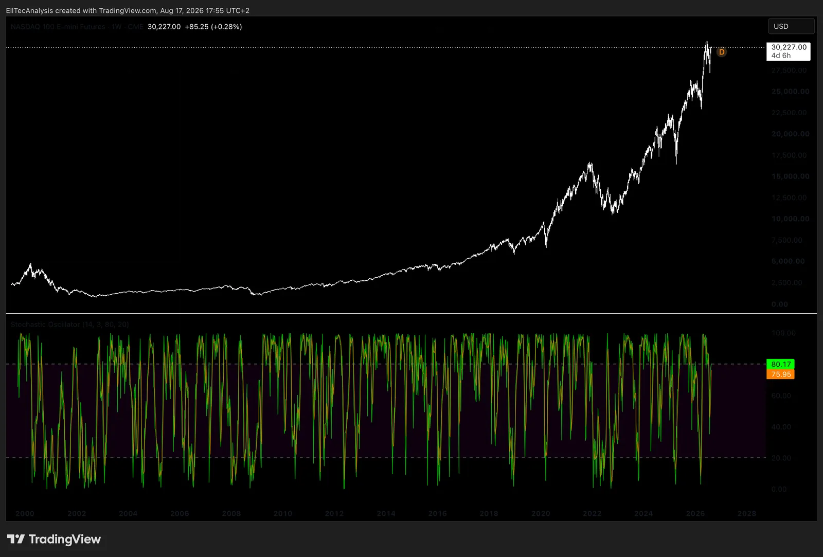
Beyond RSI and MACD, already covered below, the Stochastic oscillator applies the same overbought/oversold logic to where the current price sits within its recent trading range rather than to the speed of recent price changes. Bollinger Bands plot a volatility-based envelope around a moving average, and price touching or exceeding a band signals a statistically unusual extension relative to recent volatility, while the width of the bands themselves is a direct visual read of whether volatility is currently expanding or contracting, the same underlying concept as the volatility regimes discussed further in Part XIII. On-Balance Volume, OBV, is a cumulative running total that adds a period’s volume on an up day and subtracts it on a down day, and its value lies almost entirely in divergence: OBV failing to confirm a new price high or low is a genuine early warning that the participation behind a move is weakening, extending the same divergence logic already introduced for RSI. Average True Range, ATR, measures the average size of a security’s price movement over a lookback period in absolute terms, is not directional at all, and functions primarily as the volatility input for the ATR-based position sizing covered in Part XVII, rather than as a standalone buy or sell signal.

Valuation, Momentum, and Structure: P/E and P/B

The price-to-earnings and price-to-book ratios, along with the rest of the fundamental valuation toolkit, are covered in full in Part V; they are not repeated here since they answer a fundamentally different question, what a business is worth, rather than the price-structure and momentum questions this Part is built around.

RSI and MACD

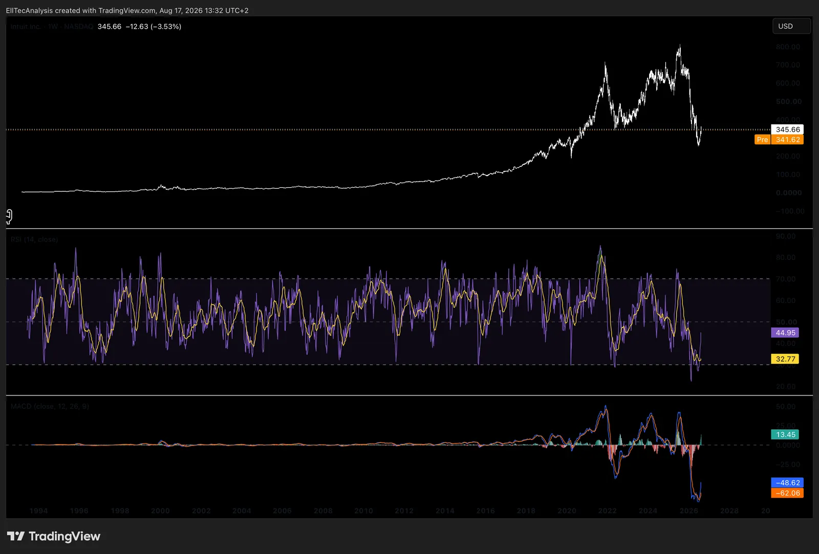
The Relative Strength Index measures the speed and magnitude of recent price changes on a zero-to-one-hundred scale, conventionally flagging readings above seventy as overbought and below thirty as oversold. RSI is most useful not as a standalone buy or sell trigger but as a divergence tool: when price makes a new high or low that RSI fails to confirm, it often signals that the move’s underlying momentum is fading before price itself turns. The Moving Average Convergence Divergence indicator tracks the relationship between two exponential moving averages of different lengths, and its crossovers and histogram are used to gauge trend direction and momentum shifts. Both are momentum tools, and both work best as confirmation for a structural view rather than as a signal generated in isolation.

Fibonacci Ratios

Fibonacci retracement and extension levels, most commonly the 38.2%, 50%, 61.8%, and 78.6% retracements and the 1.618, 2.618, and 4.236 extensions, are derived from the mathematical Fibonacci sequence and appear with striking regularity in the proportional relationships between waves of price movement across every liquid market and every timeframe. They are the mathematical backbone of Elliott Wave analysis, covered in full in Part XI: retracement levels define the probable zones where a correction is likely to complete, and extension levels define the probable zones where an impulsive move is likely to terminate. Used alone, a Fibonacci level is just a number on a chart; used within a structural wave count, it becomes a genuine probability zone with a defined invalidation point on the other side of it.

Volume and the Fixed Range Volume Profile

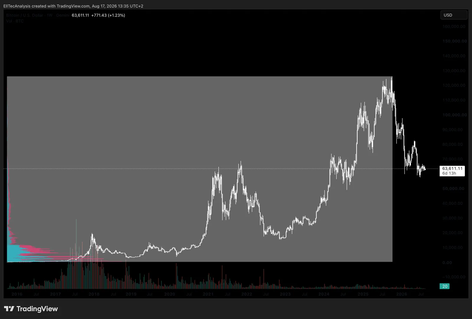
Price tells you where the market went. Volume tells you how much conviction went with it. A breakout on expanding volume carries far more structural weight than the same breakout on thin, disinterested volume, and a trend that continues while volume quietly contracts is often a trend running out of participants before it runs out of price. The Fixed Range Volume Profile takes this further by showing exactly how much volume traded at each individual price level across a chosen range, rather than over time, which reveals the price zones where the heaviest transacting occurred. Those high-volume nodes tend to act as magnets and as support or resistance later on, because they represent the price levels where the largest number of market participants established a position and therefore have the strongest incentive to defend it.

Market Breadth

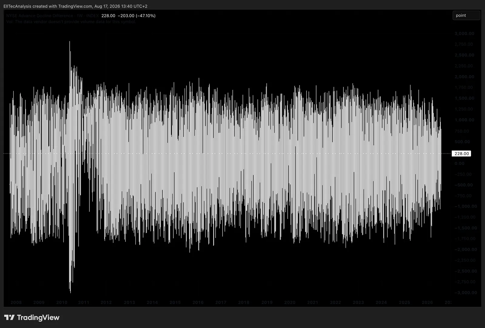
Everything covered so far in this Part reads a single security’s own price and volume. Market breadth extends the same logic to an entire index, measuring how many individual constituents are actually participating in a move rather than reading the index level alone, which can be dragged higher or lower by a handful of the largest names while the broader market underneath tells a genuinely different story. The Advance/Decline Line is the classic breadth tool: each session, the number of declining stocks is subtracted from the number of advancing stocks within an index, and that daily net figure is added to a running cumulative total. A healthy, broad-based rally sees the A/D Line make new highs alongside the index itself; a rally where the A/D Line fails to confirm a new index high, continuing to lag or even decline while the headline index grinds higher, is a classic breadth divergence, the same underlying warning already introduced for RSI and OBV, here applied at the level of the whole market rather than a single security, and it has historically been one of the more reliable early signals that a trend’s underlying participation is narrowing before the index price itself turns. New Highs and New Lows counts the number of constituents within an index hitting a fresh 52-week high or low on a given session, and the balance between the two offers the same participation read from a different angle: an index at a new high accompanied by a shrinking number of individual constituents also making new highs signals the same narrowing leadership the A/D Line would flag. Further refinements built on the same underlying data, the percentage of an index’s constituents trading above their own 200-day moving average, and the McClellan Oscillator, a smoothed momentum measure derived directly from advance/decline data, extend this same breadth logic without changing its core purpose: confirming or questioning whether a headline index move genuinely reflects the market underneath it, rather than a handful of large constituents alone.

Liquidity Heatmaps

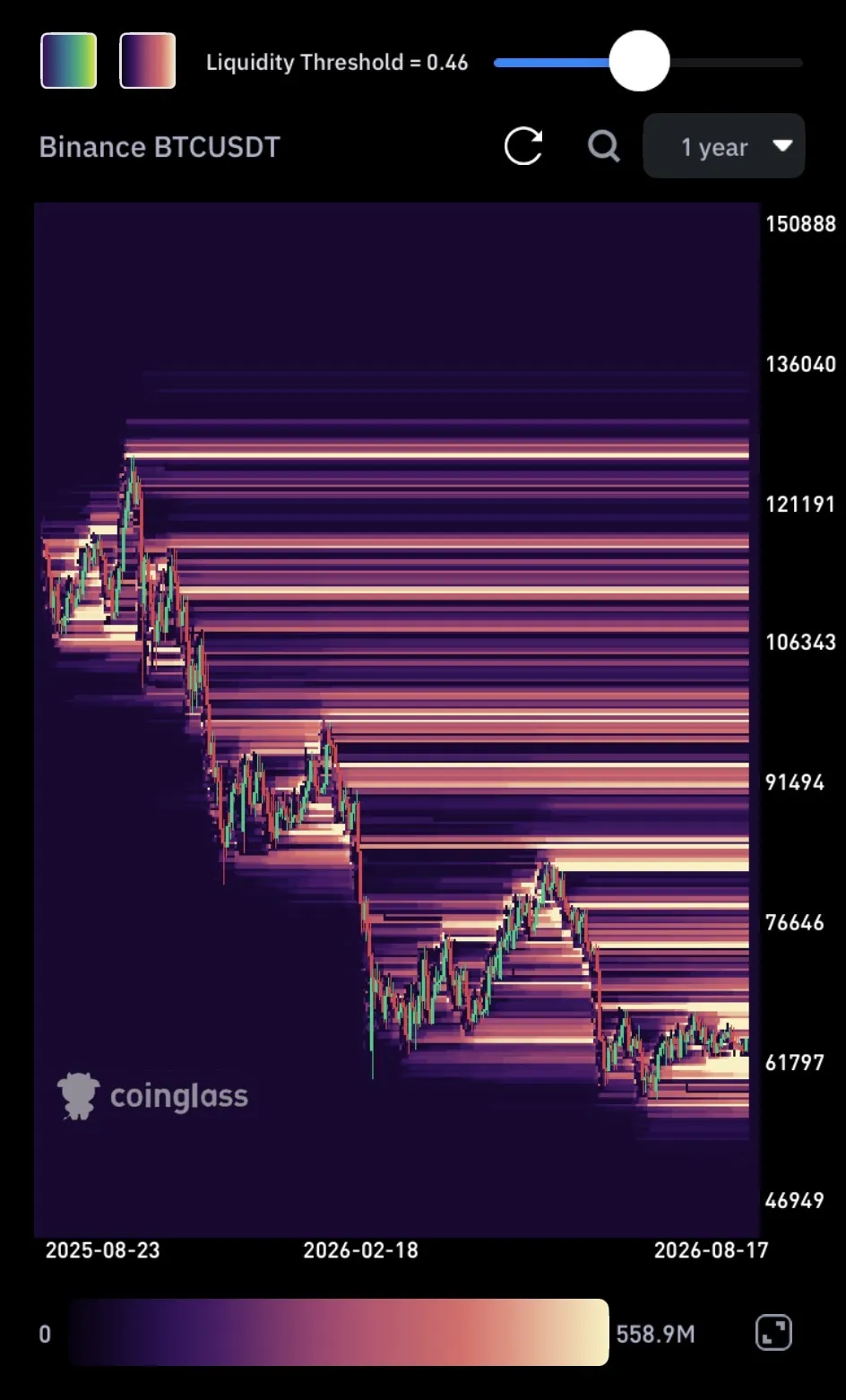
A liquidity heatmap visualises the concentration of resting limit orders across price levels on an exchange’s order book, typically displayed as a depth map that thickens where large clusters of buy or sell orders sit. These clusters often represent zones where price is statistically more likely to gravitate toward, since they concentrate the liquidity needed to fill large orders, and they can also represent zones engineered to trigger stop-loss cascades once price interacts with them. Liquidity heatmaps are a short-to-medium-term structural tool, most useful in highly liquid, order-book-driven markets such as major crypto pairs and index futures.

Leading, Lagging, and Confirmation Indicators

It is worth being explicit about what category a given tool actually falls into, since conflating them is a common source of misapplied signals. Leading indicators attempt to anticipate a move before it fully develops, RSI divergence and volume behaviour both fall into this category. Lagging indicators confirm a move after it has already begun, moving average crossovers and MACD signal-line crosses are the clearest examples, valuable for confirmation but structurally late by design. Confirmation indicators are not meant to generate an independent signal at all, but to validate a signal already generated elsewhere, volume confirming a breakout being the textbook case. No single tool in this Part is designed to work well in isolation; the philosophy behind reading several of these together, leading, lagging, and confirming, alongside the fundamental and macro backdrop covered elsewhere in this guide, is the same philosophy behind how EllTec Analysis structures every report.

Part XI: Market Sentiment and Positioning

Sentiment indicators do not predict where price goes next. They measure how crowded, or how one-sided, current positioning already is, which is most useful precisely at genuine extremes and considerably less useful as a routine, ongoing signal.

VIX and VVIX

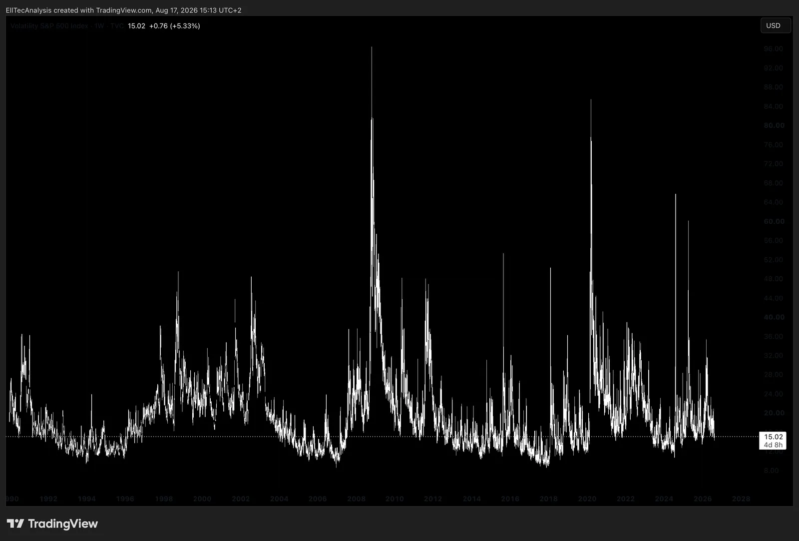
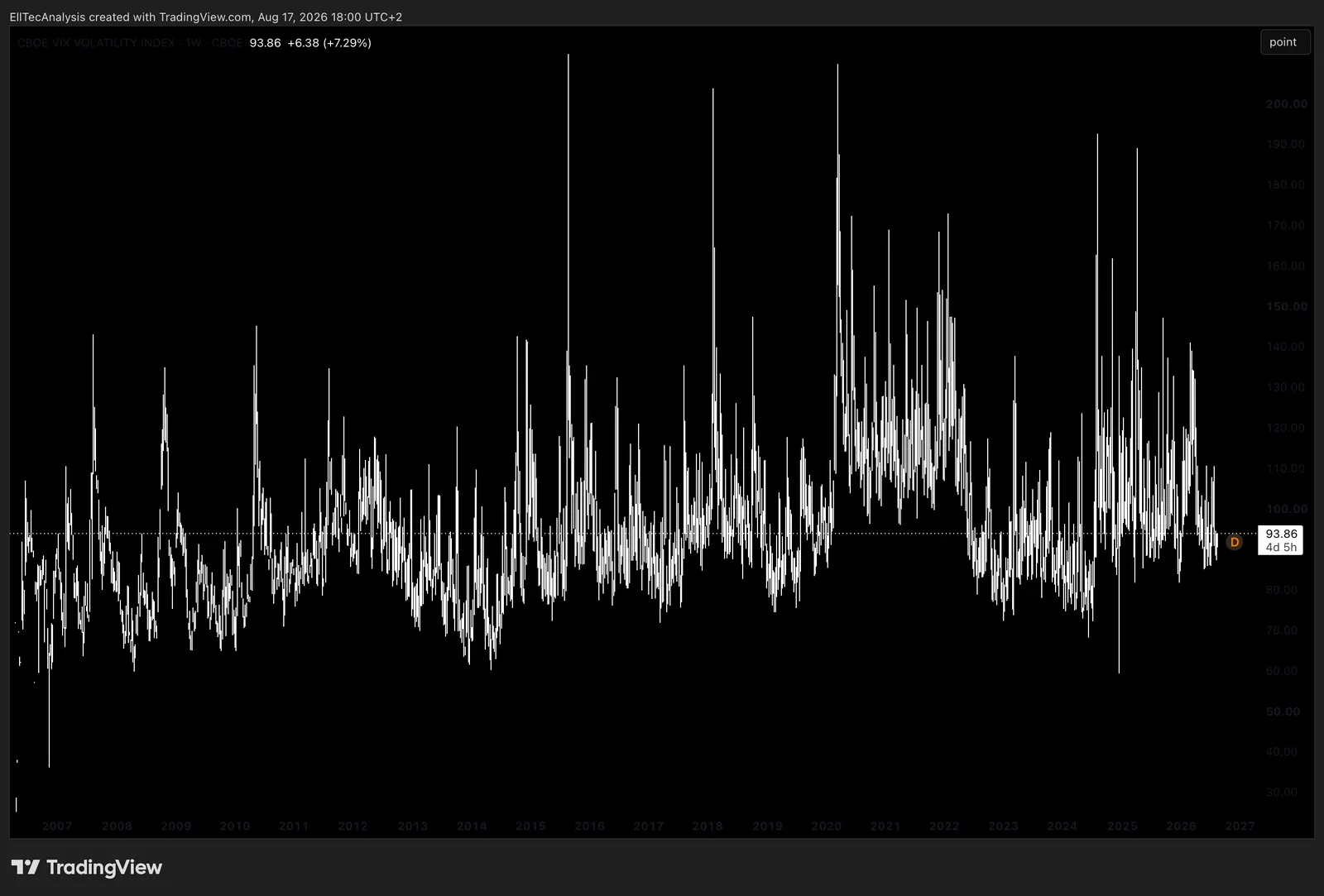
The CBOE Volatility Index, universally known as the VIX, measures the market’s expectation of 30-day forward volatility in the S&P 500, derived from option pricing. It is frequently called the market’s fear gauge: low VIX readings, broadly in the mid-to-high teens, reflect complacency and orderly markets, while sharp spikes above thirty typically coincide with genuine risk-off events. The VIX itself tends to mean-revert, which is why extreme readings in either direction are often treated as contrarian signals rather than trend confirmations. VVIX measures the volatility of the VIX itself, effectively a “vol of vol” gauge, and rises when the option market expects the VIX itself to move unpredictably, commonly ahead of major, binary macro events where the range of plausible outcomes is unusually wide.

Put/Call Ratio and Volatility Skew

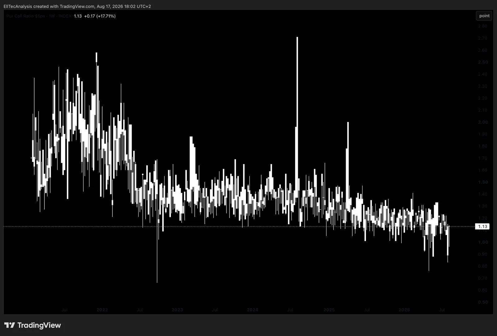
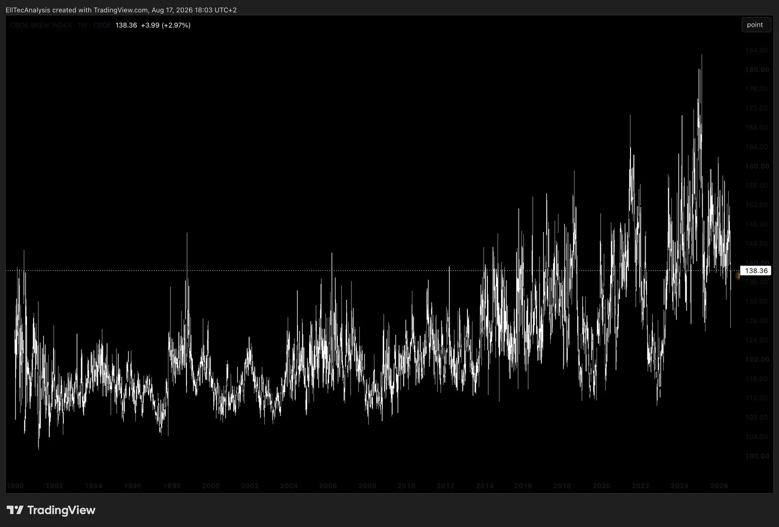
The put/call ratio compares the trading volume or open interest of put options against call options across the market, and an elevated ratio signals more hedging or outright bearish positioning is currently in place; as with the VIX, it is genuine extremes, not routine day-to-day fluctuation, that carry real contrarian information. Volatility skew, introduced in Part VII, persistently sees OTM puts priced with higher implied volatility than OTM calls in equity index options, and this reflects structural, ongoing hedging demand rather than a fresh signal at any single moment, which is exactly why a change in the level of skew is more informative than the level itself.

Dealer Gamma and Options Flow

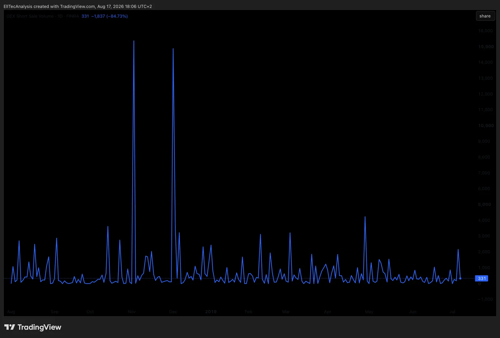
Options flow tracks unusually large or aggressive options trades as a rough proxy for informed institutional positioning. Dealer gamma, or gamma exposure (GEX), is a more mechanical and genuinely useful concept: market makers who sell options to the public must hedge their own resulting directional exposure by trading the underlying asset itself. When dealers are collectively net long gamma, a state common in calmer markets with heavy put-buying activity from the public, their hedging flows tend to dampen volatility, buying modest dips and selling modest rallies. When dealers are collectively net short gamma, their hedging flows work in the opposite, self-reinforcing direction, amplifying moves already underway, a dynamic that has contributed to some of the sharpest, fastest selloffs and squeezes in recent market history. This is a genuinely useful, if more advanced, lens for understanding why volatility itself sometimes clusters into sudden, outsized moves.

The Market Participant Landscape

Positioning and flow data means little without understanding who is actually generating it, since different participant types operate under structurally different constraints and goals that shape how they trade. Mutual funds generally face daily redemption liquidity requirements and are frequently managed against a specific benchmark, which constrains how far they can deviate from that benchmark’s composition regardless of conviction. Pension funds and insurers manage long-dated liabilities decades into the future and are correspondingly the natural buyers of the long-duration bonds covered in Part VI, often driven as much by regulatory capital and liability-matching requirements as by a pure return objective. Hedge funds operate under considerably more flexible mandates, able to go short, use leverage, and concentrate positions in ways a typical mutual fund cannot, but face their own constraint in the form of investor redemption terms, which can force a fund to sell a genuinely sound position simply to meet client withdrawals during a period of poor performance. Commodity Trading Advisors, CTAs, run largely systematic, rules-based strategies, heavily weighted toward the trend-following approach covered in Part IX, across futures markets spanning every asset class in this guide, and their collective, correlated positioning is itself a source of the momentum and trend persistence, and occasionally the sharp trend reversals, observed across markets. Recognising which type of participant is likely behind a given flow, a benchmark-constrained mutual fund rebalancing, a liability-driven pension fund extending duration, or a systematic CTA piling into an already-extended trend, adds real context to the positioning tools covered throughout the rest of this Part.

Positioning Data: Short Interest, the COT Report, and Fund Flows

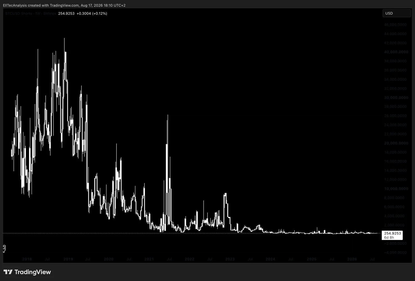
Short interest and days-to-cover, already introduced in Part IV, remain the clearest single-stock positioning gauge available to retail. At the market level, the Commitments of Traders (COT) report, published weekly by the CFTC, breaks down open positioning in US futures markets by participant type, commercial hedgers, and speculative funds, and is the closest thing retail investors have to seeing institutional futures positioning directly rather than inferring it indirectly. ETF and broader fund flows, net creation versus redemption activity across sectors, asset classes, and geographies, offer a real-time read on where capital is actually being allocated, distinct from where prices are simply moving, and the two can diverge meaningfully during a rally or selloff driven more by existing holders than by fresh buying. Margin debt, the aggregate level of leverage investors are carrying against their portfolios, is a slower-moving, structural risk gauge rather than a short-term timing tool; elevated and rapidly rising margin debt has historically coincided with more fragile market structure, since a price decline large enough to trigger widespread margin calls can force indiscriminate selling that deepens the decline itself, entirely independent of any change in underlying fundamentals.

Retail Positioning, Institutional Positioning, and Sentiment Surveys

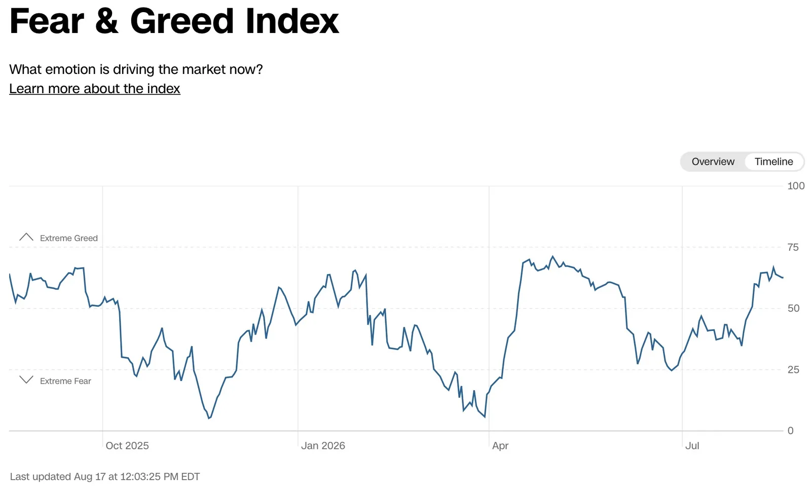
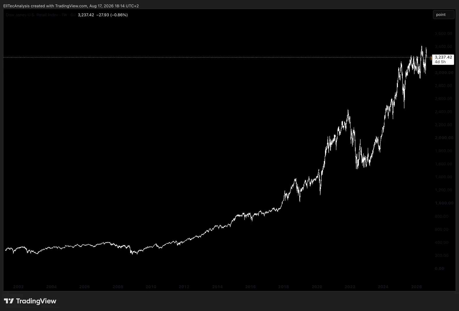
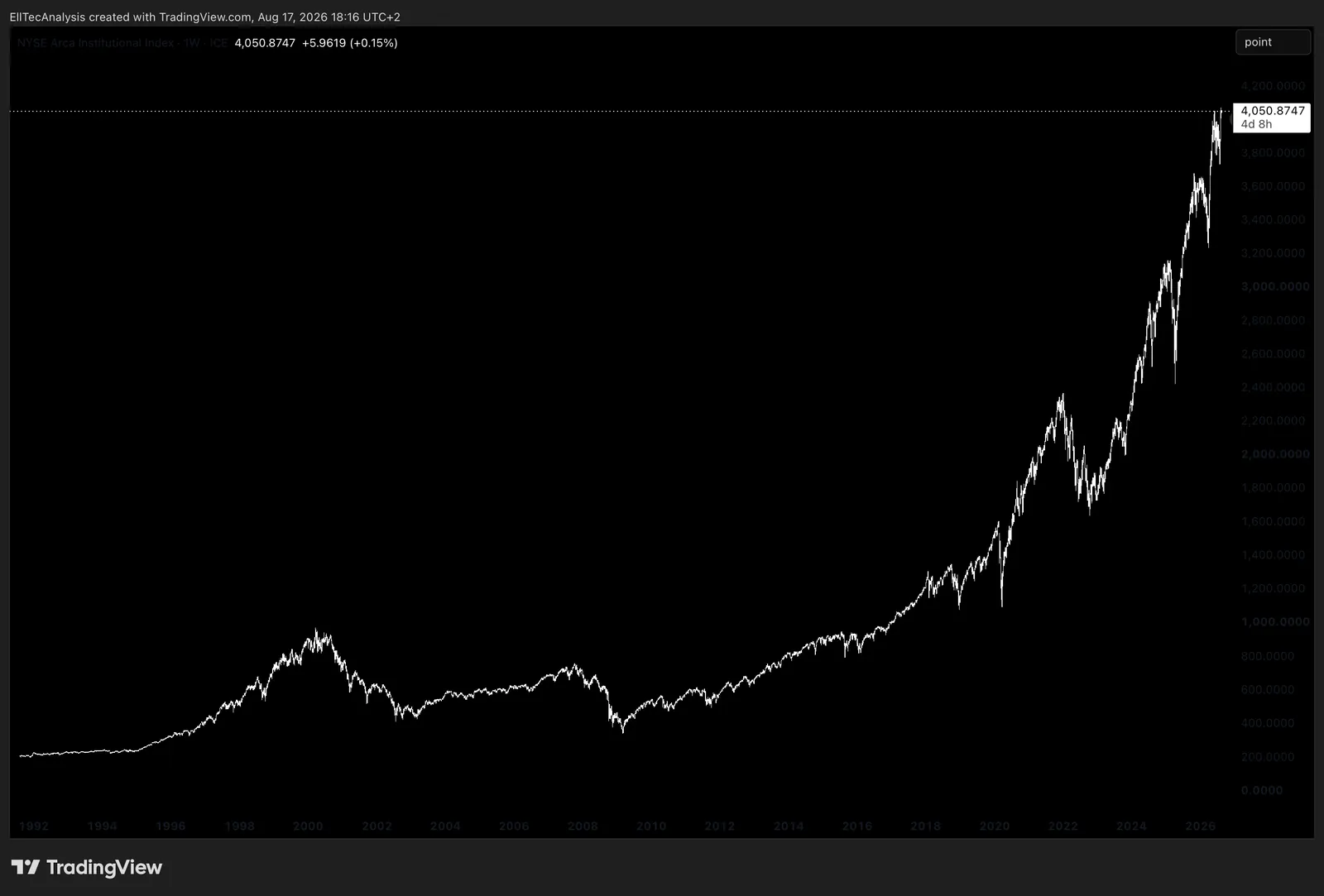
Retail and institutional positioning frequently diverge at market extremes, and general sentiment surveys, whether measuring bullish-versus-bearish respondent sentiment or the more market-derived Fear and Greed Index already covered, tend to reach their own extremes near, though rarely at the exact moment of, a market turn. Of everything covered in this Part, broad sentiment surveys are the least mechanically reliable in isolation and the easiest to over-interpret, since they measure stated opinion rather than actual capital at risk, and are best treated as one input alongside the more mechanical, positioning-based tools above rather than a standalone signal.

Crypto-Specific Positioning

Perpetual futures funding rates and aggregate open interest, the real-time gauges of how crowded and how leveraged positioning is in the crypto derivatives market specifically, are covered in full in Part XVI, alongside the liquidation dynamics that make crypto’s positioning data considerably more consequential to near-term price action than the equivalent data is in most traditional markets.

Credit Spreads as a Market-Wide Stress Gauge

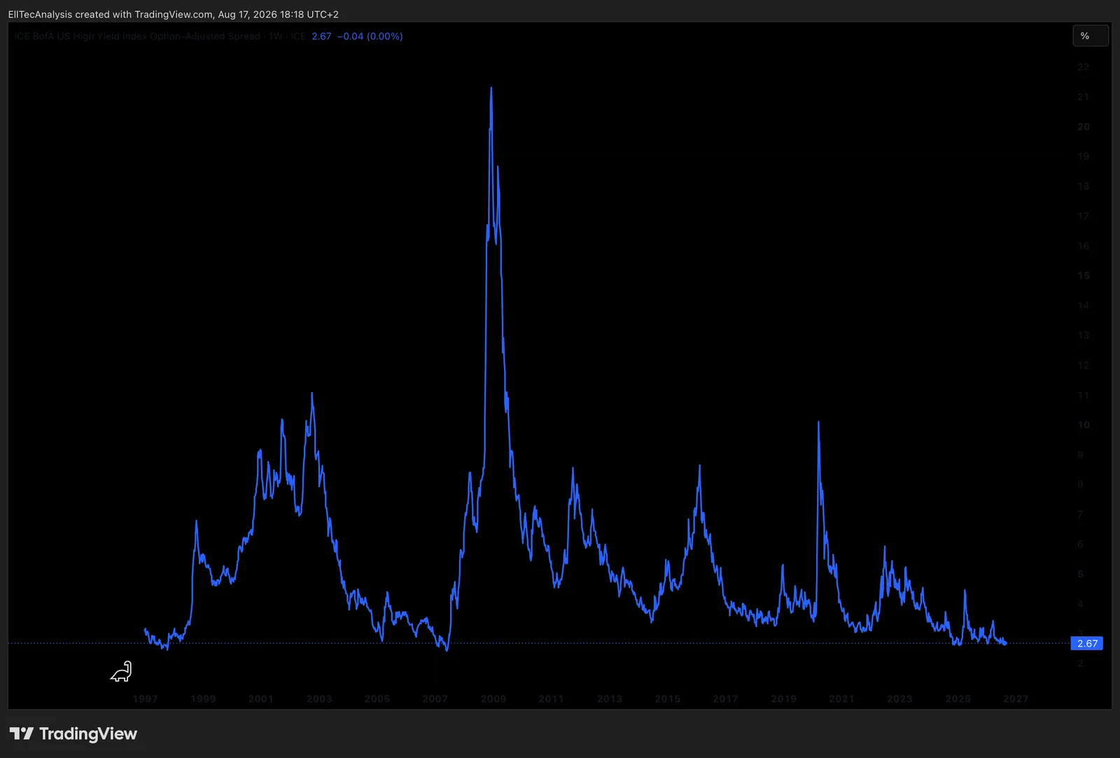
Credit spreads, defined mechanically in Part VI, double as one of the two most important cross-asset sentiment and stress gauges available at the market-wide level, alongside the VIX. The ICE BofA US High Yield Index Option-Adjusted Spread is the benchmark measure of this premium in the US market, published daily by ICE Data Indices and available free via FRED. As an illustration of what a tight reading looks like: the spread stood at roughly 271 basis points (2.71%) as of mid-August 2026, historically a low level, meaning credit markets were pricing in minimal default risk and broad financial conditions were accommodative at that time. This specific figure will have moved by the time this guide is read; what matters structurally is the mechanism, not the number. When the spread widens sharply, it signals that bond investors are pulling back from risk before equity markets typically catch up to the same conclusion, which is precisely why credit spreads are watched as a leading indicator of broader market stress rather than a lagging confirmation of it. As a rough scale for reading the level itself: spreads below roughly 350 basis points have historically signalled late-cycle complacency, while spreads above roughly 800 basis points have historically coincided with genuine recessionary stress.

Which of These Actually Matter

Genuine extremes in the VIX, the put/call ratio, and the Fear and Greed Index are useful contrarian gauges precisely because they are genuine extremes; the same tools produce far less signal during ordinary, range-bound fluctuation and should not be treated as a constant, ongoing trading input. The COT report and options flow are useful as objective, hard positioning data, but a large net position, long or short, can persist and even grow for an extended period without a reversal, so they inform probability rather than timing on their own. Margin debt is a structural, slow-moving fragility gauge, not a short-term signal. Dealer gamma is genuinely underused by retail investors relative to how much it actually explains about why volatility clusters the way it does. And broad sentiment surveys, useful as one data point among many, are the single easiest tool on this list to over-weight and should never be relied on alone.

Part XII: Macroeconomics, Economic Data, the Business Cycle, and Market Regimes

Inflation Regimes

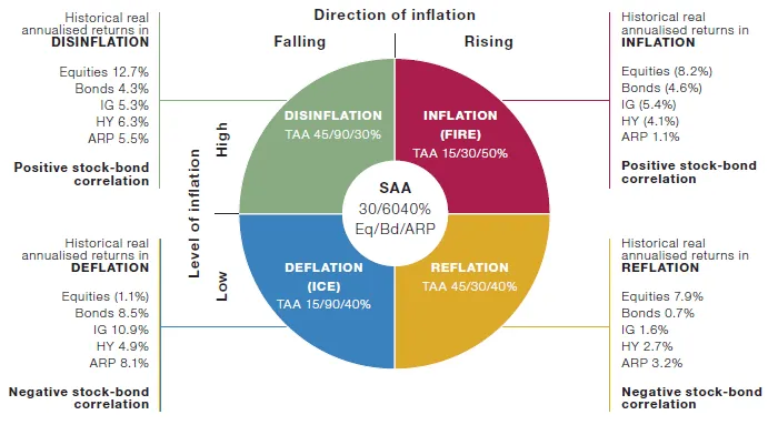
These five terms are frequently used loosely, and the distinctions between them carry real consequences for markets. Inflation is a general, sustained rise in prices across the economy. Deflation is a general, sustained fall in prices, and it is generally treated as more damaging to an economy than moderate inflation, since falling prices encourage consumers and businesses to delay spending in anticipation of even lower prices later, and they mechanically raise the real burden of any existing fixed-rate debt. Disinflation is not deflation; it describes inflation that remains positive but is decelerating, prices are still rising, simply more slowly than before, a distinction worth holding onto since the two are commonly and incorrectly conflated in casual market commentary. Reflation describes a deliberate, policy-driven effort to push growth and inflation back up from a depressed or negative level, typically following a recession, using both monetary and fiscal tools together. Stagflation, high inflation combined with stagnant growth and elevated unemployment occurring simultaneously, is the single hardest regime for a central bank to manage, since the standard tool for fighting inflation, raising rates, actively worsens growth and unemployment, and the standard tool for supporting growth, cutting rates, actively worsens inflation.

Monetary and Fiscal Policy

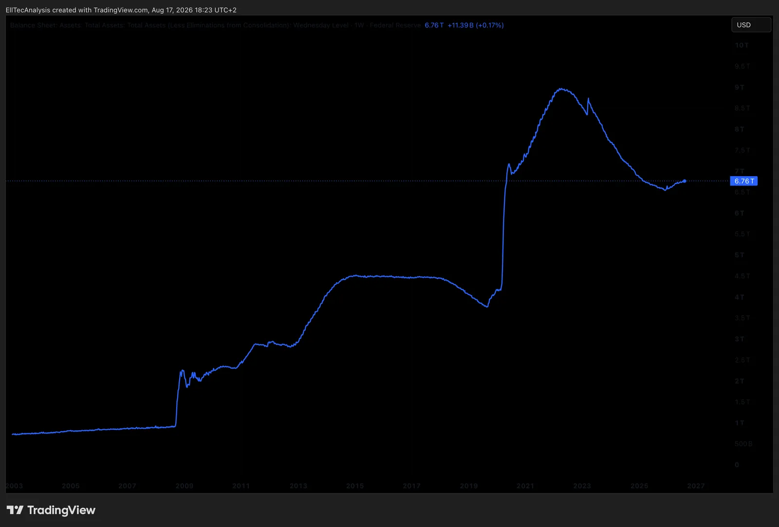
Monetary policy is the central bank’s own toolkit: the policy rate covered in Part I, quantitative easing, QE, the outright purchase of government and other bonds to inject liquidity and hold longer-term yields down when the policy rate alone has limited room left to move, and quantitative tightening, QT, the reverse, allowing the balance sheet built up through QE to shrink, which drains system liquidity, expanded further below. Forward guidance, a central bank’s explicit or implied communication about its likely future policy path, is itself a policy tool, since markets price in expectations well ahead of an actual rate decision, which is why a rate decision that matches expectations exactly can still move markets sharply if the accompanying guidance surprises. Fiscal policy is a separate lever entirely, government spending and taxation decisions made by elected authorities rather than the central bank, and the two can reinforce each other, expansionary fiscal policy alongside accommodative monetary policy, or work directly against each other, a central bank tightening rates specifically to offset inflationary pressure created by a large fiscal deficit. One well-known framework for judging where policy “should” sit is the Taylor Rule, which prescribes a policy rate based on how far inflation sits from its target and how far output sits from its potential; no central bank follows it mechanically in practice, but it remains a useful conceptual anchor for judging whether current policy looks loose or tight relative to the prevailing economic backdrop.

The Yield Curve, Real Yields, and Breakeven Inflation

The yield curve’s shape and its historical relationship to recessions is covered mechanically in Part VI; at the macro level, an inversion is watched specifically as a signal that the market expects the central bank to be cutting rates in the future in response to weaker growth, which is precisely why short rates trading above long rates has preceded most modern recessions, while never functioning as an infallible, mechanically certain trigger. Real yields, the nominal yield minus expected inflation, matter more than nominal yields for judging the actual restrictiveness of financial conditions and for valuing risk assets, since a nominal yield that looks high can still be historically loose in real terms if inflation expectations are high enough to match it. Breakeven inflation, the market-implied inflation expectation calculated as the gap between a nominal government bond’s yield and the yield of an equivalent-maturity inflation-linked bond covered in Part VI, is the market’s own real-time forecast of future inflation, distinct from and often more current than a backward-looking inflation data release.

Money Supply, Bank Reserves, and Central Bank Balance Sheets

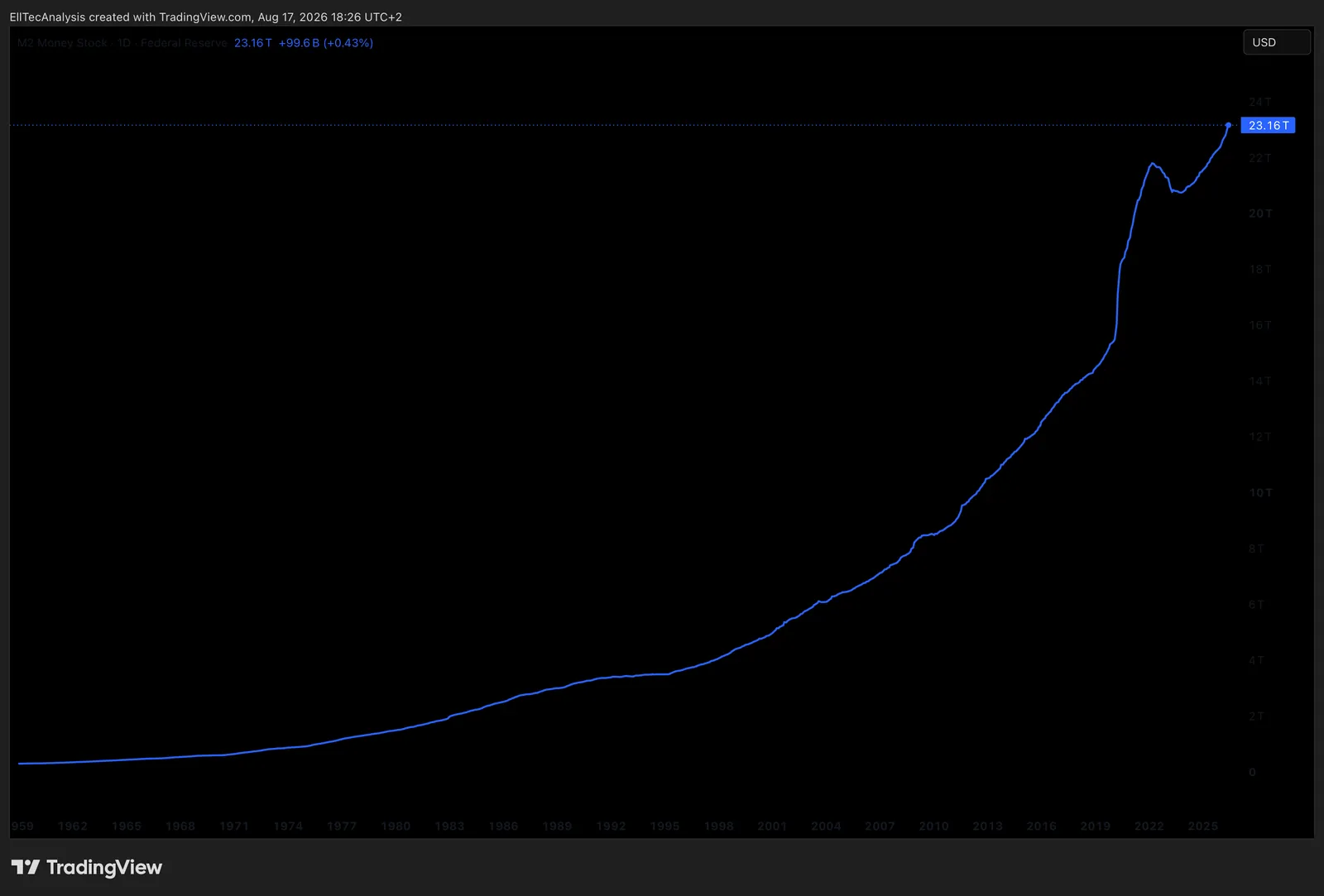
M2, a broad measure of money supply covering cash, checking and savings deposits, and other readily accessible funds, is watched as a gauge of aggregate liquidity in the financial system, though the relationship between M2 growth and subsequent inflation has proven considerably less mechanical and predictable in practice than simple monetarist theory once suggested. Bank reserves, the deposits commercial banks hold at the central bank, expand directly through the QE process already described, and central bank balance sheet size, the aggregate value of assets a central bank holds on its books, both broadly track and shape the amount of system-wide liquidity available in the same expanding-or-contracting direction already established above. Bank lending and credit creation, the pace at which commercial banks actually extend new loans into the real economy, is the mechanism through which central bank policy ultimately reaches businesses and households, and a central bank can hold policy accommodative while bank lending standards independently tighten, producing an economy that still feels credit-constrained despite loose headline policy. Financial conditions indices combine several of these inputs, rates, credit spreads, equity volatility, and the dollar, into a single composite gauge of how loose or tight the overall backdrop currently is, often a more complete picture than any single input alone. Dollar liquidity, the availability of US dollar funding globally, and the DXY, the US Dollar Index measuring the dollar against a basket of major currencies, matter well beyond US borders, since a large share of global trade and debt is dollar-denominated; a sharply strengthening dollar mechanically tightens financial conditions for the rest of the world, particularly for emerging markets carrying dollar-denominated debt, a dynamic revisited directly in Part XIV.

Interest Rates

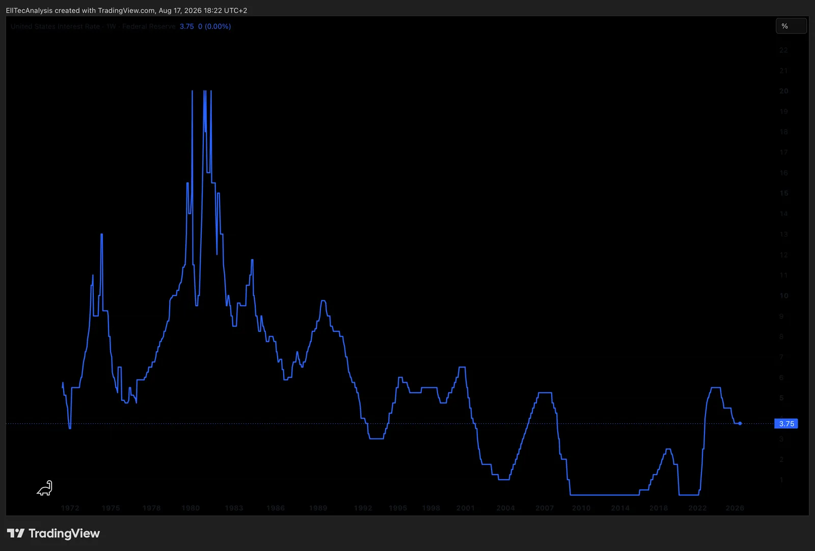
The policy rate set by the central bank is the single most important price in the entire financial system, because every other asset is ultimately valued relative to the risk-free rate, and Treasury yields across the curve form the actual benchmark against which every other borrowing cost and every DCF discount rate in Part V is ultimately anchored. As an illustration: the Federal Reserve’s target range stood at 3.50% to 3.75% as of mid-August 2026 (source: Federal Reserve, see Sources), a level that could have changed by the time this guide is read; the mechanism described below, not this specific number, is what stays evergreen. Higher rates raise the discount rate applied to future corporate cash flows, which compresses equity valuation multiples, particularly for long-duration growth companies whose earnings are weighted furthest into the future; they also raise borrowing costs across the economy, which slows growth with a lag. Falling rates work in the opposite direction, supporting valuations and easing financing conditions. The path of rates, and market expectations for that path priced into futures curves, is a more important driver of asset prices over the medium term than almost any single company or sector-level development.

Government Debt and Fiscal Sustainability

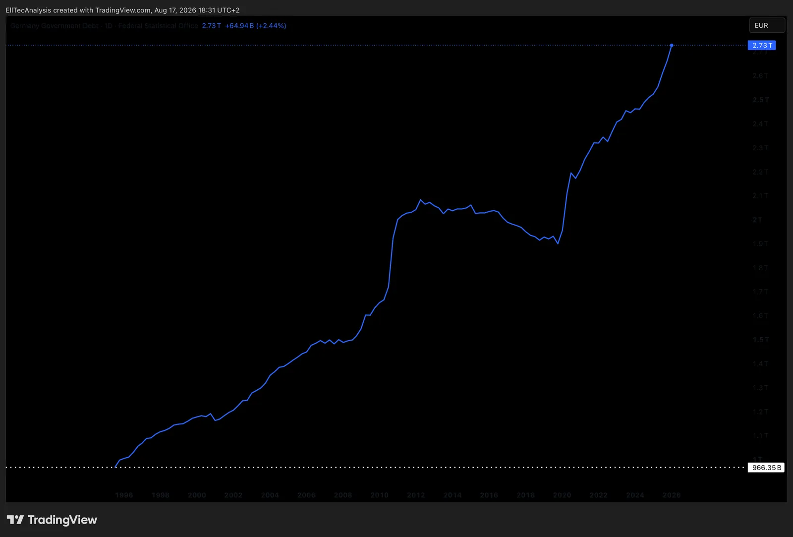
Rising government debt and persistent fiscal deficits are not automatically destabilising on their own; what matters is debt sustainability, whether an economy’s growth rate and borrowing costs allow that debt to be serviced and gradually stabilised as a share of the economy over time, or whether it compounds unsustainably. A rising deficit financed at low borrowing costs during strong growth is a materially different situation than the same deficit financed at high borrowing costs during weak growth, even though the headline debt figures might look similar.

Recession Indicators: Leading, Coincident, and Lagging

Economic data is worth sorting by timing, not just by topic. Leading indicators attempt to signal where the economy is headed before it gets there: the yield curve, PMI surveys, and initial jobless claims are the clearest examples. Coincident indicators move roughly in step with current economic activity: GDP and industrial production fall into this category. Lagging indicators only confirm what has already happened, often well after the fact: the unemployment rate is the textbook example, since employers typically continue hiring for a period after growth has already started slowing, and only cut headcount once the slowdown is confirmed.

Global Central Banks

The Federal Reserve operates under a dual mandate, price stability and maximum employment, giving it explicit latitude to weigh growth and jobs alongside inflation in its decisions. The European Central Bank operates under a single primary mandate, price stability, a structural difference that can produce a genuinely different policy reaction function to the same economic data than the Fed’s, and it sets policy for the entire eurozone through a system of national central banks rather than a single country. The Bank of England targets inflation directly, operating in a smaller, more open economy where currency moves feed through to inflation more quickly than in the US. The Bank of Japan has historically run a far more persistently accommodative policy than its developed-market peers, including extended periods of yield curve control, capping government bond yields directly rather than only setting a short-term policy rate, a structurally different toolkit from the others on this list. The People’s Bank of China manages a broader and less purely rate-based toolkit than Western central banks, including reserve requirement ratios for banks and more direct administrative guidance, alongside active management of its currency, reflecting a financial system with materially different structure and openness than the others covered here.

How Macro Transmits Into Each Asset Class

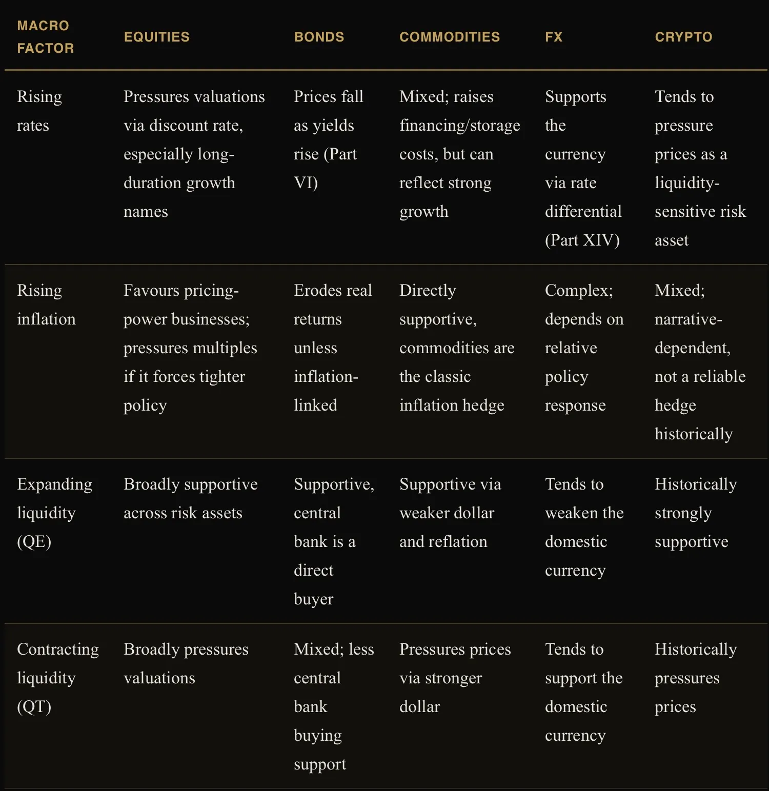
The Business Cycle in Depth

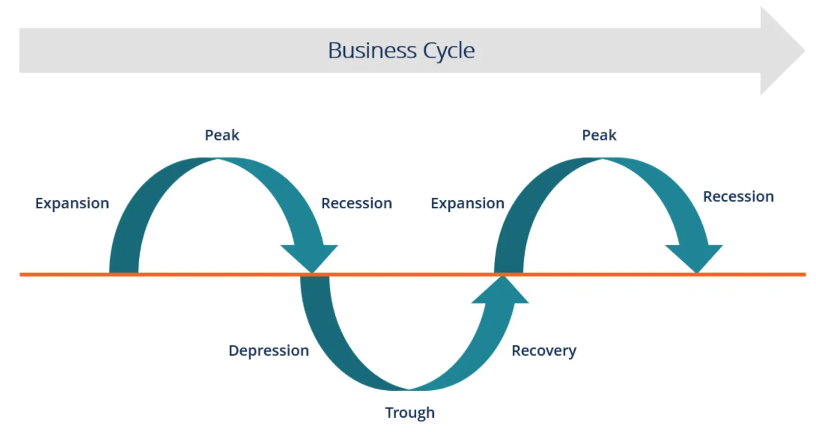
The economy moves through a recurring, if irregular, sequence: expansion (growth accelerating from a trough), peak (growth at its maximum rate, beginning to decelerate), contraction (growth slowing or turning negative), and trough (the cycle’s low point, setting up the next expansion). Expansion itself is commonly split into early, mid, and late phases, each with a different character: early-cycle growth is typically the fastest and most broad-based, mid-cycle growth moderates but remains healthy, and late-cycle growth is decelerating with inflation pressure often building as the economy runs closer to full capacity. A recession is formally associated with a sustained contraction in broad economic activity; a soft landing describes inflation successfully brought under control without triggering a recession, the most favourable and least common outcome; a hard landing describes the opposite, a recession triggered as the cost of bringing inflation down.

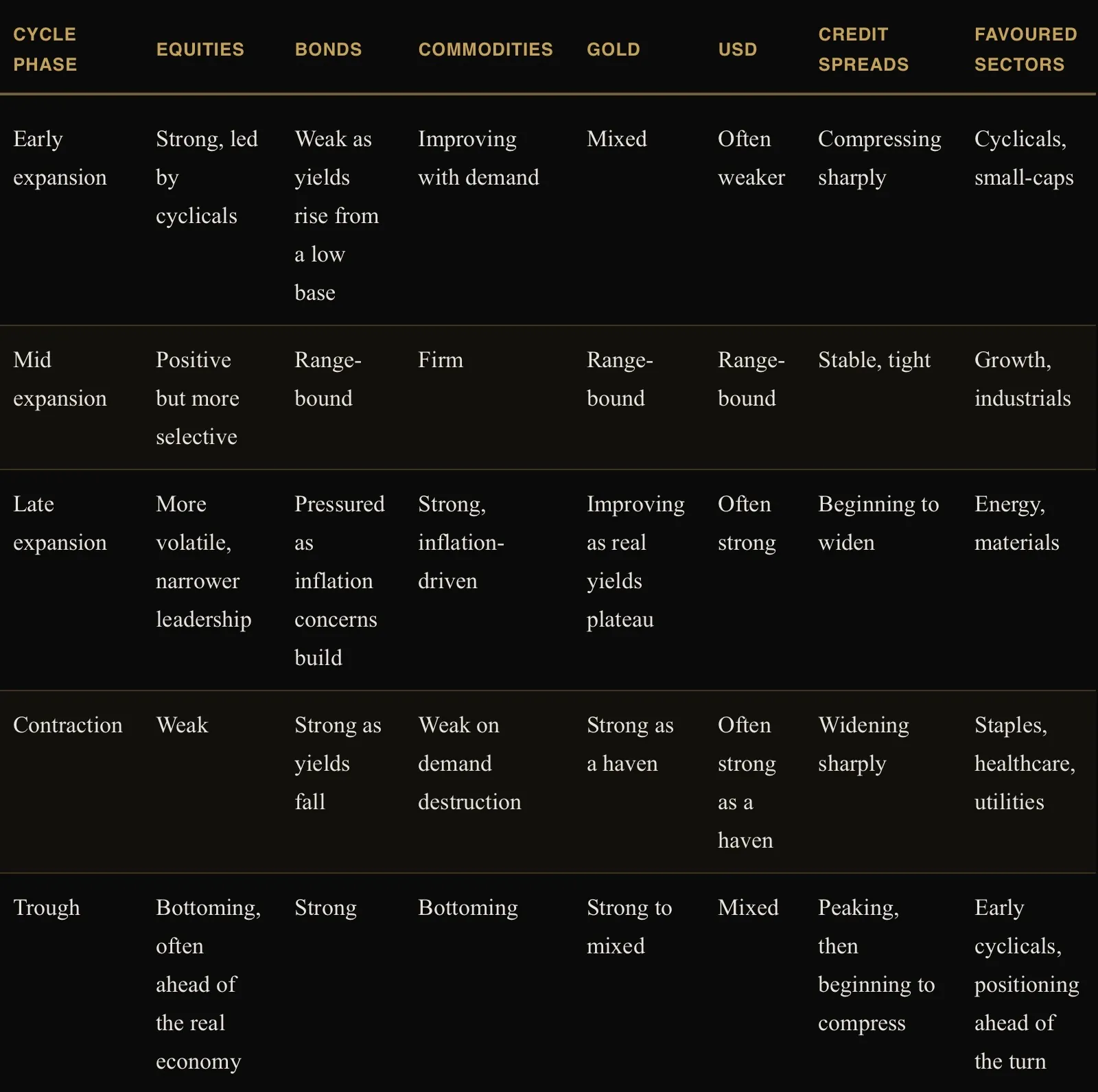
None of this is a mechanical formula. Cycles vary considerably in length and severity, and policy intervention has repeatedly stretched or compressed phases that historically played out over years into a matter of months. But understanding roughly where the cycle currently sits provides essential context for weighing which asset classes and sectors carry the wind at their back and which are working against the macro tide, which is precisely the top-down layer that sits underneath every EllTec Analysis report before the technical structure is even considered.

Correlation

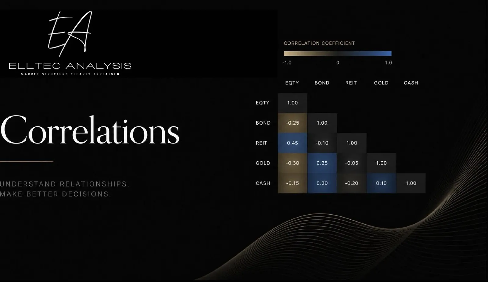
Correlation measures how closely two assets move together, expressed on a scale from minus one, perfectly opposite, to plus one, perfectly in lockstep. Correlations are not fixed constants. They regime-shift, and the shift usually happens exactly when investors need diversification most, during systemic stress, when asset classes that normally move independently suddenly move together and a portfolio that looked diversified on paper turns out to carry a single, concentrated risk. Watching correlation is therefore not an academic exercise but a direct check on whether a portfolio’s diversification is real or illusory at this specific moment in the cycle, and it is the mechanism underneath every relationship described in the intermarket analysis below.

Intermarket Analysis

Markets do not move independently of each other, and reading the relationships between them is often more informative than reading any single market alone. The classic stocks-versus-bonds relationship is typically inverse, bonds rallying when equities sell off on growth fears, though this relationship can break down and even flip positively correlated during inflation-driven selloffs, when both asset classes are pressured by the same rising-discount-rate force at once, exactly the scenario flagged in Part I. Real yields and gold move inversely, since gold pays no yield of its own and competes directly with real yields for a place in a portfolio; rising real yields raise the opportunity cost of holding a non-yielding asset like gold, and falling real yields lower it. Treasury yields and growth stocks are similarly inversely linked through the DCF mechanism in Part V: since a larger share of a growth company’s value sits further into the future, its valuation is mechanically more sensitive to the discount rate than a mature, cash-generative value stock’s is. The US dollar and commodities typically move inversely, since commodities are globally priced in dollars and a stronger dollar makes them more expensive for holders of every other currency, mechanically pressuring demand. Credit spreads and equities are tightly linked, covered further in Part XII’s discussion of the ICE BofA US High Yield OAS as a leading cross-asset stress gauge, since bond investors, as senior claimants, frequently reprice credit risk before equity investors, as residual claimants, fully catch up to the same conclusion. System liquidity and crypto move together closely, consistent with crypto’s behaviour as a genuinely liquidity-sensitive risk asset rather than the independent, uncorrelated hedge it is sometimes marketed as. Copper, sometimes called “Dr. Copper” for its diagnostic reputation, is watched as a real-time gauge of global industrial demand and, by extension, global economic growth, given its use across construction, manufacturing, and infrastructure worldwide.

Market Regimes

The same indicator, and the same strategy, can produce genuinely different results depending on the prevailing regime, and treating any tool in this guide as having one fixed, constant meaning is a mistake worth correcting explicitly. A regime is simply the prevailing character of the market or the macro backdrop along a given dimension, and several distinct dimensions matter at once. The directional regime is a bull market (a sustained uptrend), a bear market (a sustained downtrend, commonly defined once a decline reaches roughly 20% from a recent high), or a sideways, range-bound market with no sustained direction either way. The volatility regime is high or low, independent of direction entirely, describing how large the typical price swing currently is, and is read directly off the VIX and ATR levels covered in Parts XII and X. The inflation regime, already defined earlier in this Part, is high or low inflation, or the disinflationary, reflationary, or stagflationary variants covered above. The rate regime is high or low relative to recent history, already covered in the Interest Rates subsection. The liquidity regime is expansion, a QE-driven backdrop of increasing system liquidity, or contraction, a QT-driven backdrop of tightening liquidity, both already defined above. And the growth regime is a recession, a soft landing, or the hard-landing and stagflation scenarios already introduced, layering the business cycle directly on top of all of the above.

Trend-following strategies, covered in Part IX, thrive in a strong directional regime and are whipsawed repeatedly in a sideways, range-bound one; mean-reversion strategies show the mirrored pattern, thriving in range-bound conditions and getting run over in a powerful trend. An RSI reading pinned above seventy means something different in a strong, established uptrend, where it can remain elevated for an extended period without the overbought reading resolving into a reversal, than it does in a choppy, range-bound market, where the same reading has historically marked a much more reliable local top. A given level of credit spread carries a different implication two quarters into an expansion than it does two quarters into a contraction, even at an identical absolute basis-point reading.

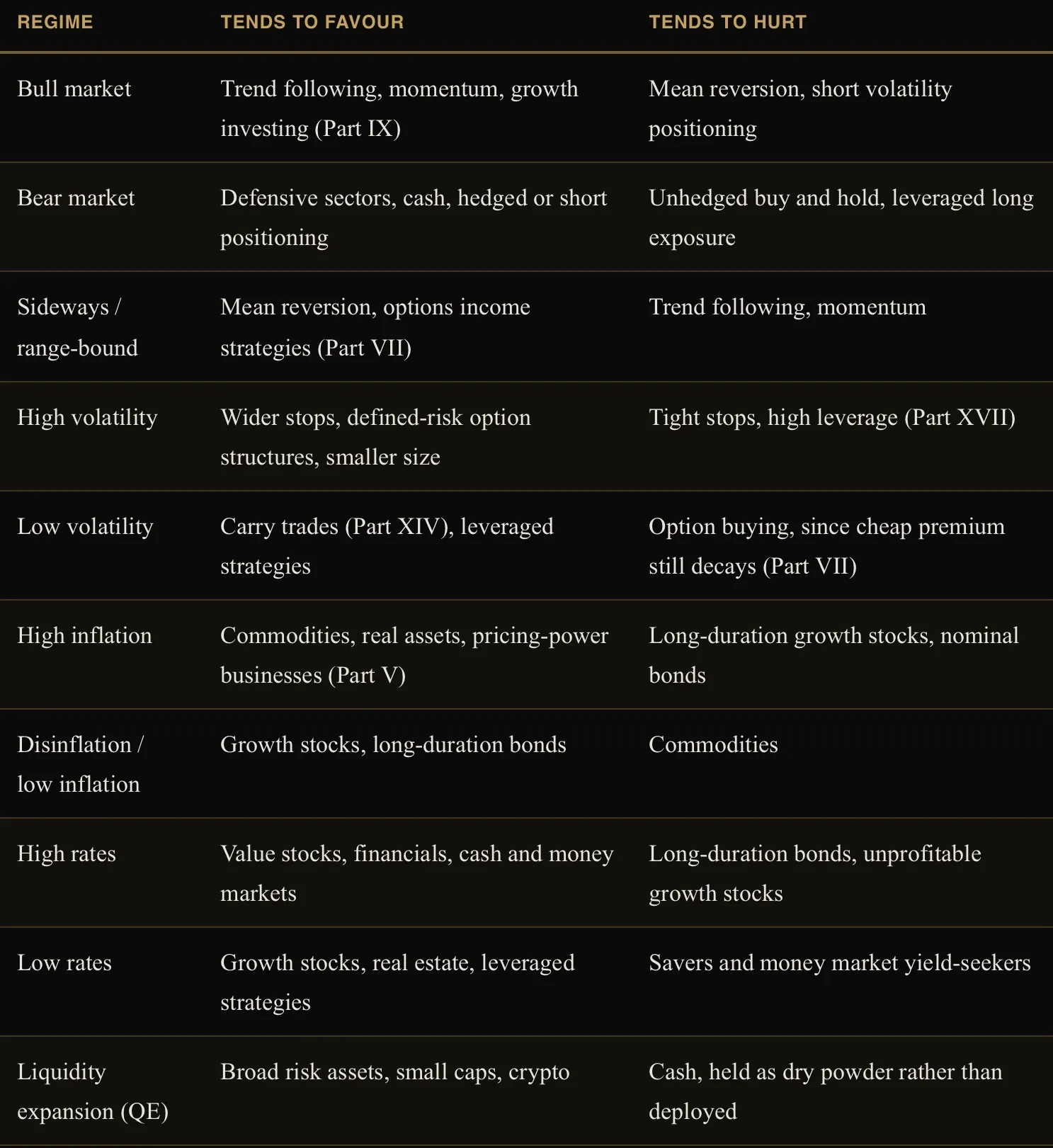
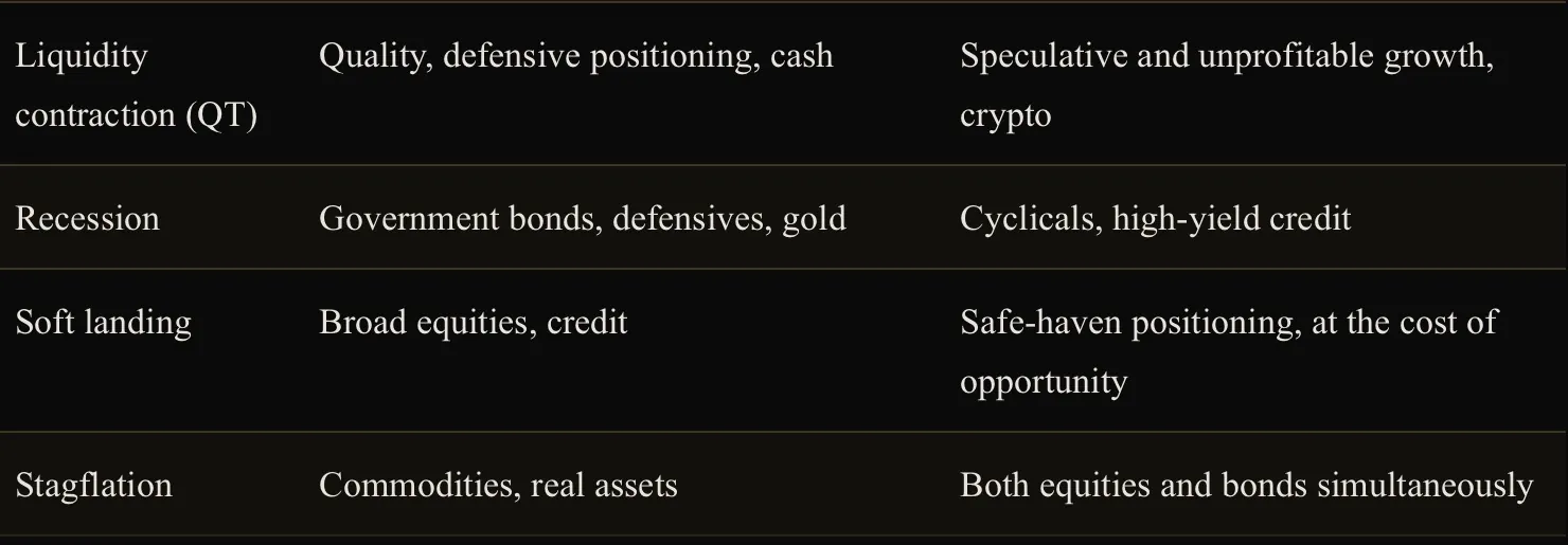
Recognising which regime currently applies, across each of these dimensions at once, before applying any tool from earlier in this guide, is not an optional extra step; it is what turns a static list of indicators into something that can actually be read correctly in the moment.

Part XIII: FX in Depth

Currency Pairs and Pips

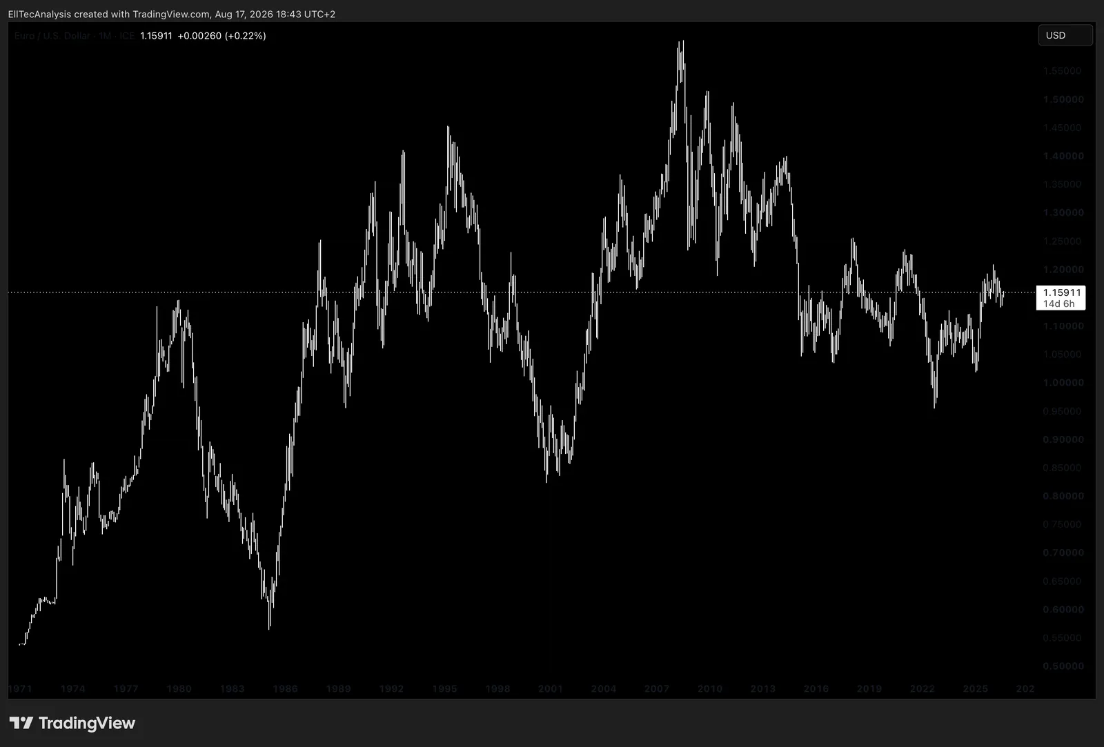
A currency pair quotes one currency, the base currency, in terms of another, the quote currency; EUR/USD at 1.16 means one euro buys 1.16 US dollars. A pip is the smallest standard unit of price movement quoted for a pair, generally the fourth decimal place for most major pairs, and the actual monetary value of a pip depends on the position size and the pair being traded. The bid-ask spread, already covered structurally in Part III, tends to be exceptionally tight for the most liquid major pairs and widens considerably for less-traded emerging market currencies.

Interest Rate Differentials, the Carry Trade, and PPP

Interest rate differentials between two countries are the primary force behind sustained currency trends, as already established in Part I, and the carry trade is the strategy built directly on top of that fact: borrowing in a low-yielding currency and investing the proceeds in a higher-yielding one, earning the rate differential as long as the exchange rate itself does not move against the position enough to erase it. Carry trades are fundamentally risk-on positions, since they depend on stable or improving risk appetite, and they are vulnerable to sudden, sharp unwinds precisely when volatility spikes and the funding currency rallies as capital rushes back to safety, which tends to happen quickly and without much warning. Purchasing Power Parity, PPP, is the long-run theoretical anchor suggesting exchange rates should adjust over time to equalise the price of an identical basket of goods across countries; it is a genuinely useful very-long-run valuation reference and a notoriously unreliable tool for anything resembling short or medium-term timing.

Central Bank Divergence and Real Rates

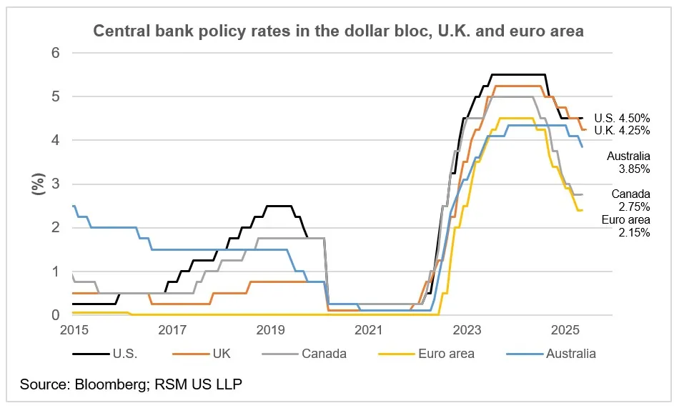
When two central banks’ policy paths diverge, one holding or cutting while the other hikes, that divergence itself becomes a primary, sustained driver of the currency pair between them, extending the macro transmission mechanism covered in Part XIII directly into FX. As with every other asset class covered in this guide, real rather than nominal rates matter more for judging genuine currency strength, since a high nominal yield offering little real return after inflation offers considerably less underlying support to a currency than the headline rate alone would suggest.

DXY and Safe-Haven Currencies

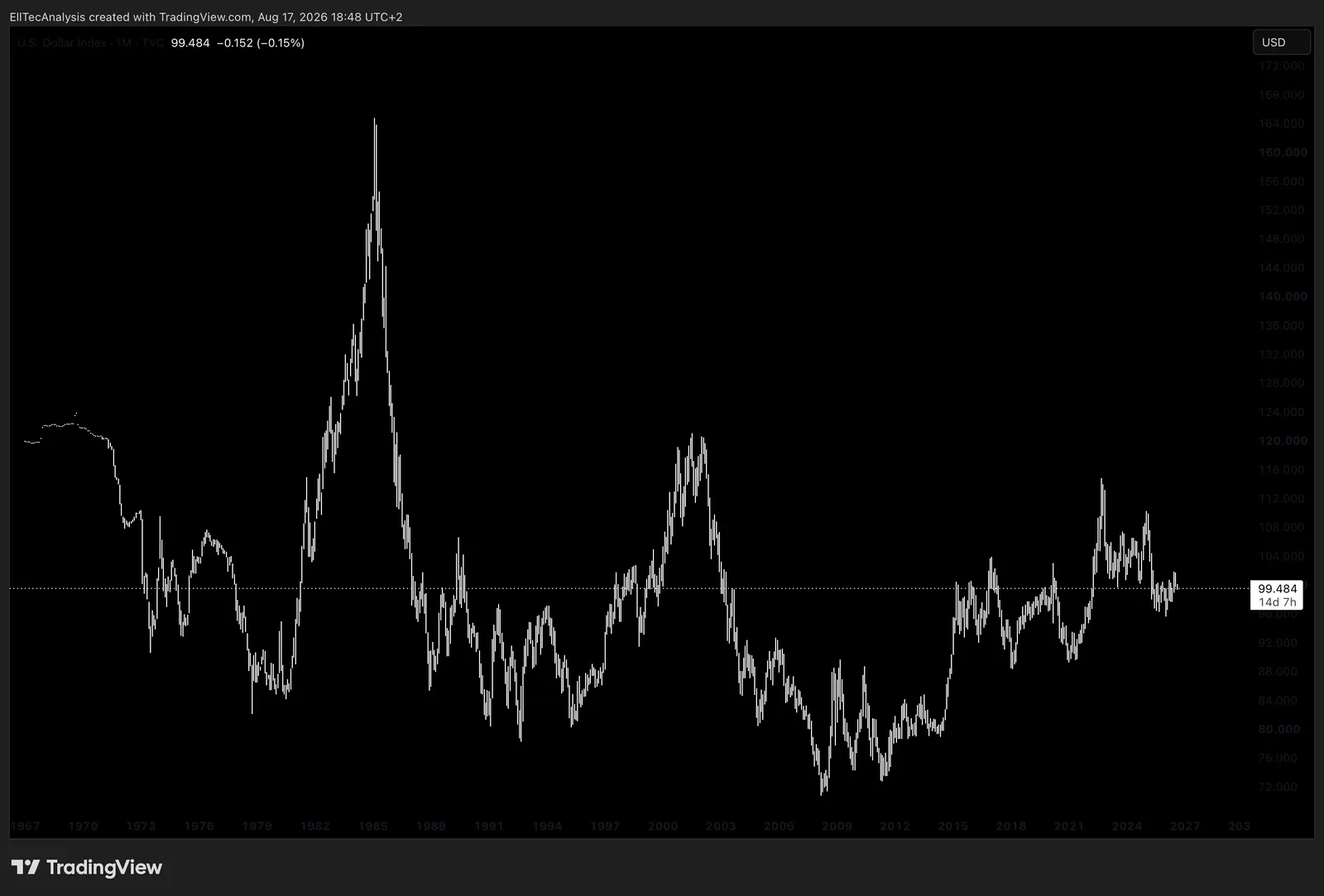
The DXY, the US Dollar Index measuring the dollar against a basket of major trading partner currencies, is the standard benchmark for gauging broad dollar strength, already introduced in Part XIII’s discussion of dollar liquidity. Certain currencies, historically the US dollar, the Japanese yen, and the Swiss franc, have tended to strengthen specifically during periods of market stress, a flight-to-quality dynamic driven by their deep, liquid government debt markets and, in Japan’s and Switzerland’s cases, their status as major net creditor nations.

Emerging Market FX

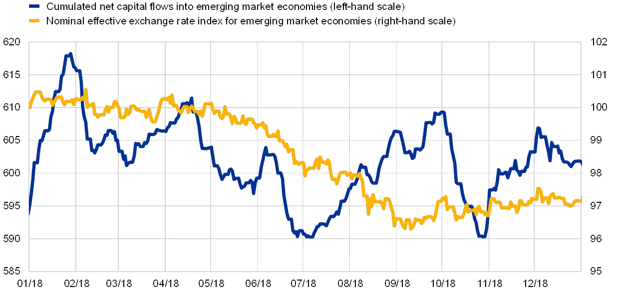
Emerging market currencies carry risk layers beyond the interest-rate and growth dynamics that drive developed-market pairs: current account deficits (a country persistently importing more than it exports, requiring ongoing foreign capital inflows to fund the gap), heavy dollar-denominated debt (which becomes proportionally more expensive to service whenever the local currency weakens against the dollar, the same transmission mechanism covered in Part XIII), and genuine political and institutional risk, all of which can trigger rapid capital flight and outsized currency moves that developed-market FX rarely experiences to the same degree.

Currency Hedging

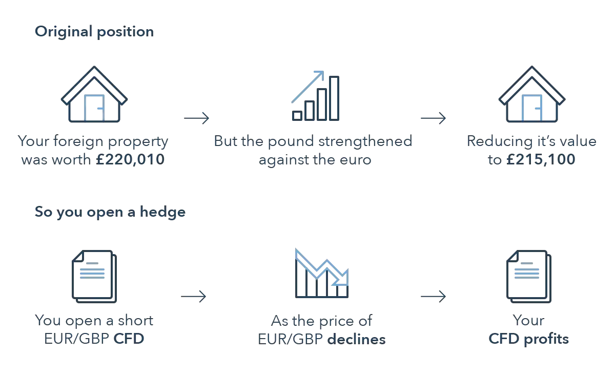
Currency hedging removes some or all of the FX translation effect from a foreign holding, typically through forward contracts or currency-hedged share classes of the kind already introduced in Part VIII’s ETF discussion. Hedging is not free: its ongoing cost is driven directly by the interest rate differential between the two currencies involved, meaning hedging a position denominated in a currency with meaningfully higher rates than the investor’s own base currency carries a real, continuous cost.

Worked Example: How FX Alone Changes a Foreign Return

Consider a EUR-based investor who buys a US stock at $100 when EUR/USD trades at 1.10, meaning the position costs roughly €90.91. Six months later, the stock is still exactly $100, unchanged in USD terms, but EUR/USD has moved to 1.05, meaning the dollar has strengthened against the euro. That same $100 position is now worth roughly €95.24 when converted back. The investor has earned a real, EUR-denominated gain of over four percent purely from the currency move, despite the underlying US stock having delivered a flat USD return. Had EUR/USD instead moved the other way, to 1.15, the same unchanged $100 stock would have translated to a EUR loss. This is exactly why an unhedged foreign holding carries a second, entirely separate return driver layered on top of the asset’s own native-currency performance, and why the hedged-versus-unhedged decision in Part VIII is not a minor technicality for any investor holding assets outside their own base currency.

Part XIV: Commodities in Depth

Spot, Futures, and the Curve

The spot price is the price for immediate delivery; the futures price is the price agreed today for delivery at a specified future date, and the mechanics of contango, backwardation, roll yield, and basis are covered structurally in Part VII. Applied specifically to commodities, the shape of the futures curve is driven by two forces beyond simple rate-based financing cost: storage cost, the real, physical expense of holding a barrel of oil or a bushel of wheat until a future date, which pushes the curve toward contango, and convenience yield, the practical benefit of holding physical inventory in hand right now rather than a paper claim on future delivery, valuable to an end user who needs the physical commodity for actual production and genuinely at risk of a supply disruption, which pushes the curve toward backwardation when current supply is tight. Inventory levels are the single most direct real-world driver of which of these two forces dominates at any given time: low inventories relative to demand tend to produce backwardation, while ample or growing inventories tend to produce contango.

Seasonality and Weather

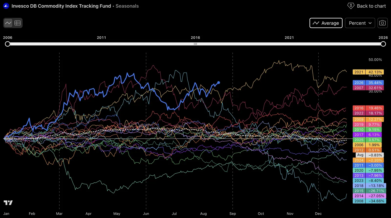
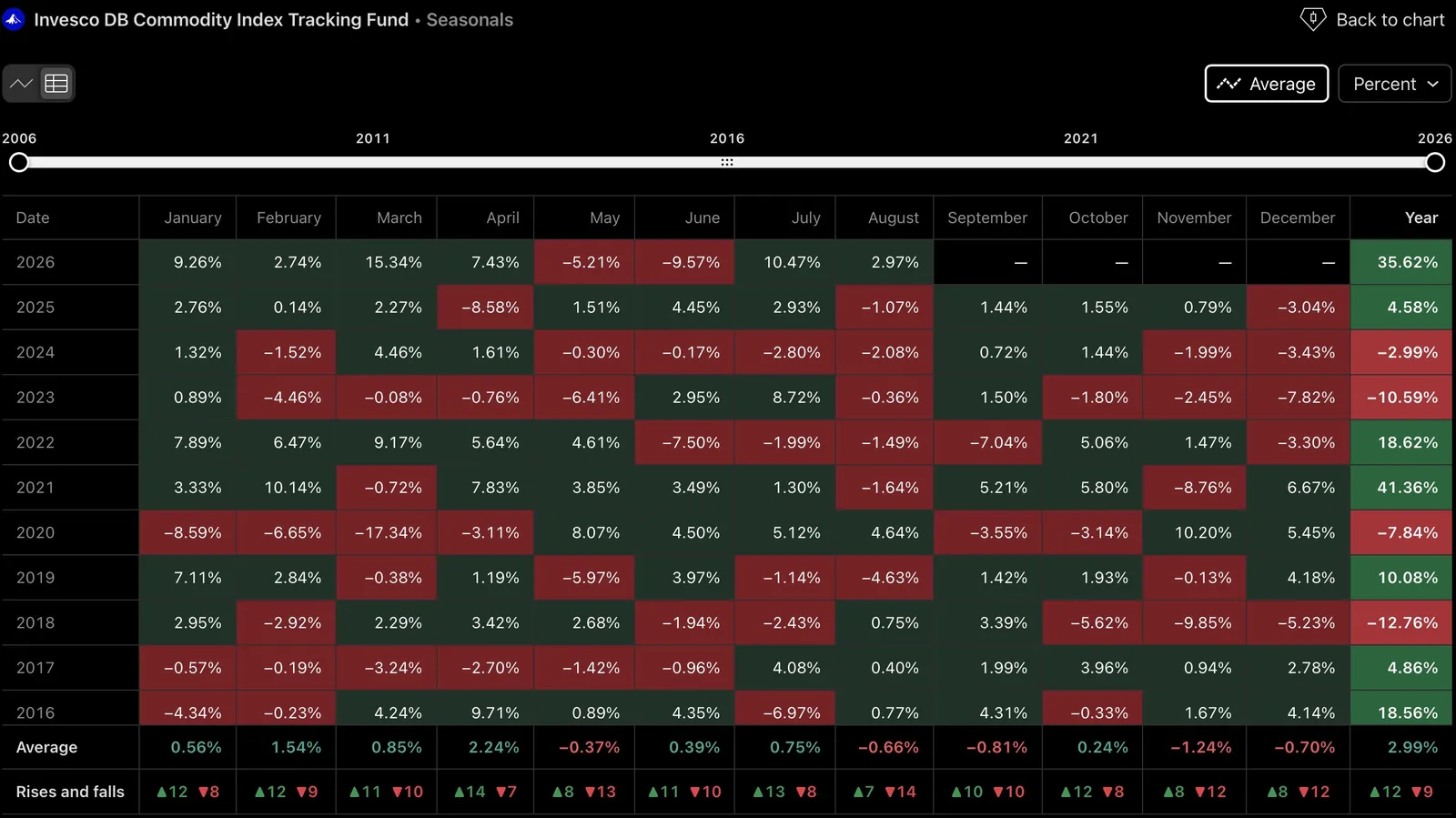
Agricultural commodities move on a genuinely seasonal rhythm tied to planting and harvest cycles, with prices typically most sensitive to weather risk during the growing season when the eventual harvest size is still uncertain. Energy commodities carry their own seasonal demand pattern, natural gas demand rising through winter heating season, gasoline demand rising through the summer driving season, and unexpected weather events, an unusually cold snap or a hurricane disrupting production infrastructure, can move prices sharply and quickly regardless of the underlying supply-demand trend.

Geopolitics, OPEC, and Demand Destruction

OPEC and its allied producers coordinate supply decisions specifically to manage the price of oil, making their meetings and production quota decisions a recurring, calendar-driven source of volatility distinct from ordinary market-driven supply and demand. Geopolitical supply shocks, conflict or sanctions affecting a major producing region, can remove meaningful supply from the market with little warning. Demand destruction is the self-correcting mechanism on the other side of a sustained price spike: sufficiently high prices eventually reduce consumption itself, whether through consumers and businesses cutting usage or substituting toward alternatives, which is part of why extreme commodity price spikes have historically tended to be self-limiting over time rather than sustained indefinitely.

Commodity Supercycles

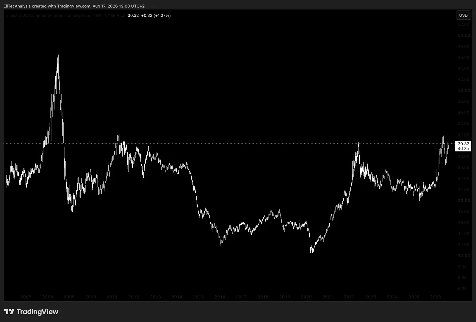
A supercycle is a multi-year, sometimes multi-decade, structural bull market across the broad commodity complex, historically driven by a sustained structural shift in demand, rapid industrialisation in a major economy being the clearest historical example, that outpaces the multi-year lead time required to bring meaningful new supply online. Recognising a genuine supercycle apart from an ordinary cyclical rally matters precisely because the investment horizon and conviction required to hold through the inevitable sharp interim corrections differ considerably between the two.

Producers Versus the Commodity Itself

Investing in a commodity-producing company, a miner or an oil major, is a meaningfully different exposure than investing in the commodity itself. Producer equities carry direct operational leverage to the commodity price, since a company’s costs are largely fixed while its revenue moves with the commodity, which amplifies both gains and losses relative to the commodity’s own return, the same operating-leverage mechanism introduced in Part V, layered on top of ordinary company-specific and equity-market risk that has nothing to do with the commodity at all.

Why a Commodity ETC Rarely Matches the Spot Price

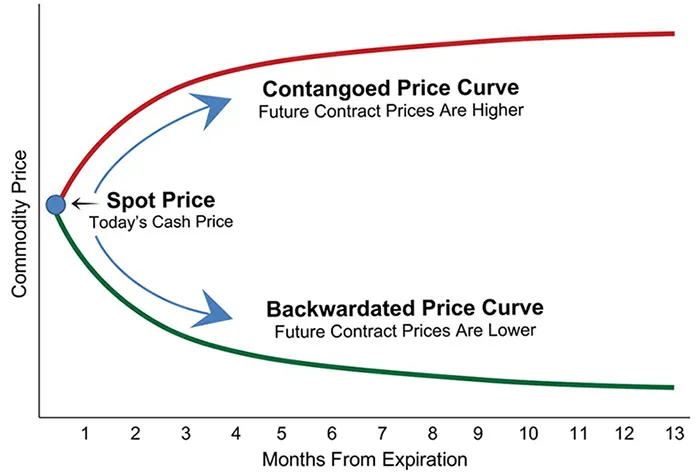
This is worth stating plainly, since it is one of the most common points of confusion for retail investors in this asset class. Most commodity ETCs do not hold the physical commodity; they hold futures contracts and must continuously roll expiring contracts into new ones to maintain exposure, which means the roll yield mechanism from Part VII, positive in backwardation, negative in contango, becomes a direct, ongoing drag or tailwind on the ETC’s realised return, entirely independent of what the spot price itself does. An ETC can post a meaningfully worse return than the spot commodity’s own price change over the same period purely from a persistently contangoed curve, which is exactly why checking a commodity ETC’s actual construction and roll methodology matters as much as checking which commodity it claims to track.

Part XV: Crypto Market Structure in Depth

Network Architecture

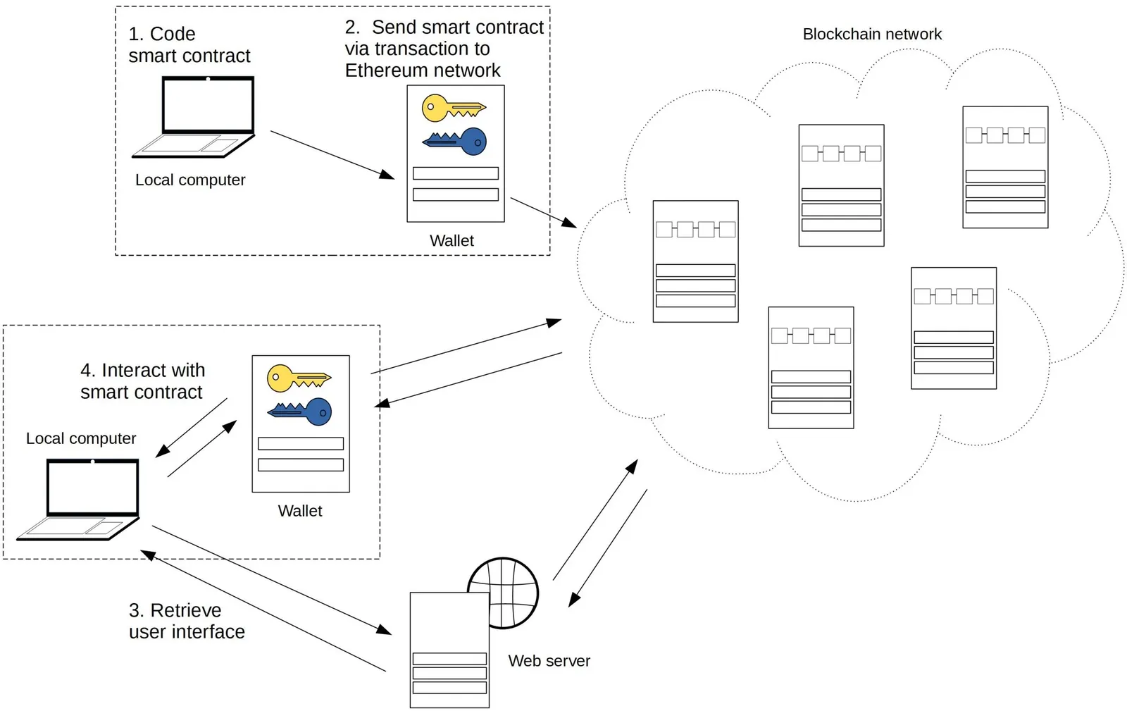
A Layer 1 is a base blockchain with its own independent consensus mechanism, Bitcoin and Ethereum being the two largest examples. A Layer 2 is built on top of a Layer 1 specifically to increase transaction throughput and reduce fees, while still inheriting the base layer’s underlying security. Rollups are the dominant current Layer 2 technique: they bundle, or “roll up,” a large batch of transactions off the base chain and then post a single, compressed proof of that batch back to the Layer 1, dramatically reducing the cost per transaction while still ultimately settling on the more secure base layer. Bridges connect separate blockchains or a Layer 1 to its Layer 2s, allowing assets to move between otherwise incompatible networks, and bridges have historically been among the single largest sources of loss in the entire crypto ecosystem, since they concentrate a large pool of locked assets behind what is often less battle-tested code than the underlying base-layer protocols themselves.

DeFi, Staking, and Tokenomics

Decentralised Finance, DeFi, refers to lending, borrowing, and trading protocols that run directly on smart contracts rather than through a traditional financial intermediary. Staking, introduced structurally in Part I, locks tokens to help secure a Proof of Stake network in exchange for a yield, a return source genuinely distinct from price appreciation and one that carries its own risk, since staked tokens are typically illiquid for a lockup period and the underlying token’s price can still fall by more than the yield earned. Tokenomics, a token’s overall economic design, determines how sustainable that design actually is. Circulating supply is the number of tokens currently in public circulation; fully diluted valuation, FDV, is what the total market capitalisation would be if every token that will ever exist were already in circulation at the current price, and the gap between a token’s market cap and its FDV is a critical, frequently overlooked check, since a token with a large share of its eventual supply still locked can look inexpensive on market cap alone while carrying substantial future dilution baked in. Token unlocks and vesting schedules are the scheduled release of previously locked tokens, typically held by the founding team and early investors, and because these dates are known in advance, they frequently create a predictable, anticipated source of future selling pressure. Some networks continuously issue new tokens as part of their ongoing security or reward mechanism, an inflationary force on supply, while others burn, permanently destroy, a portion of tokens through their normal operation, a deflationary force; the net of issuance and burns, not either figure in isolation, determines whether actual circulating supply is growing or shrinking over time.

Network Usage and On-Chain Data

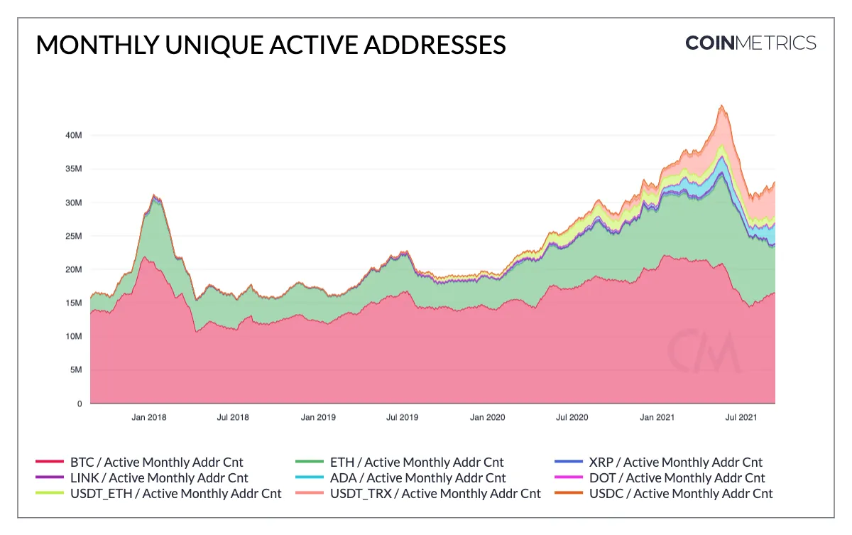
Gas fees are the cost of executing a transaction on a network, and they rise and fall directly with demand for the network’s limited block space, functioning as a real-time congestion gauge. Total Value Locked, TVL, is the aggregate value of assets deposited into a network’s DeFi protocols and is widely used as a rough proxy for that ecosystem’s genuine, organic usage. Active addresses, transaction volume, and network fees collected all serve a similar purpose, distinguishing networks with real, sustained activity from those whose token price is being driven by speculation with comparatively little underlying usage behind it, and developer activity, the pace of ongoing code contribution to a network’s core protocol, is a further proxy for its long-term health and prospects. Exchange flows, the net movement of a token onto or off centralised exchanges, are watched as a positioning signal: large inflows to exchanges often precede selling, since an exchange is where a token is actually sold, while large outflows toward self-custody often signal longer-term holding intent. Whale activity, tracking the wallets known to hold unusually large positions, offers a similar, if noisier, positioning read.

Perpetual Futures, Funding Rates, Open Interest, and Liquidations

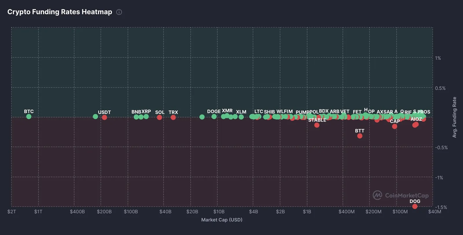
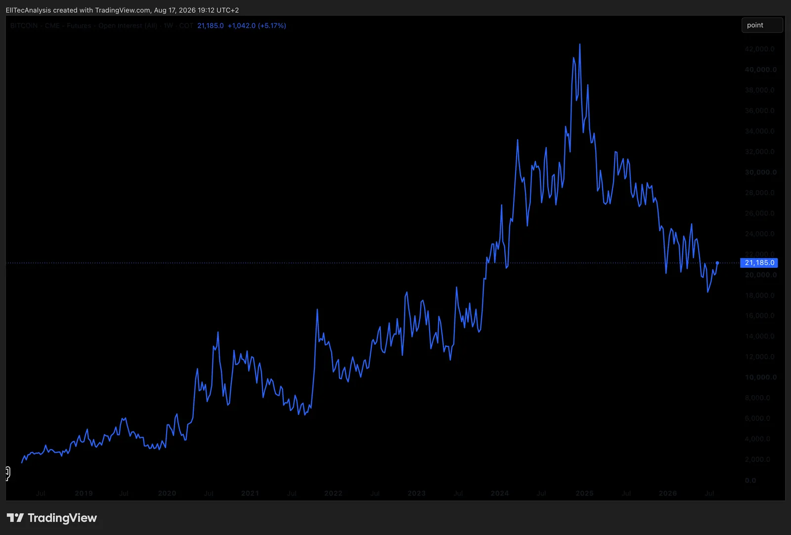
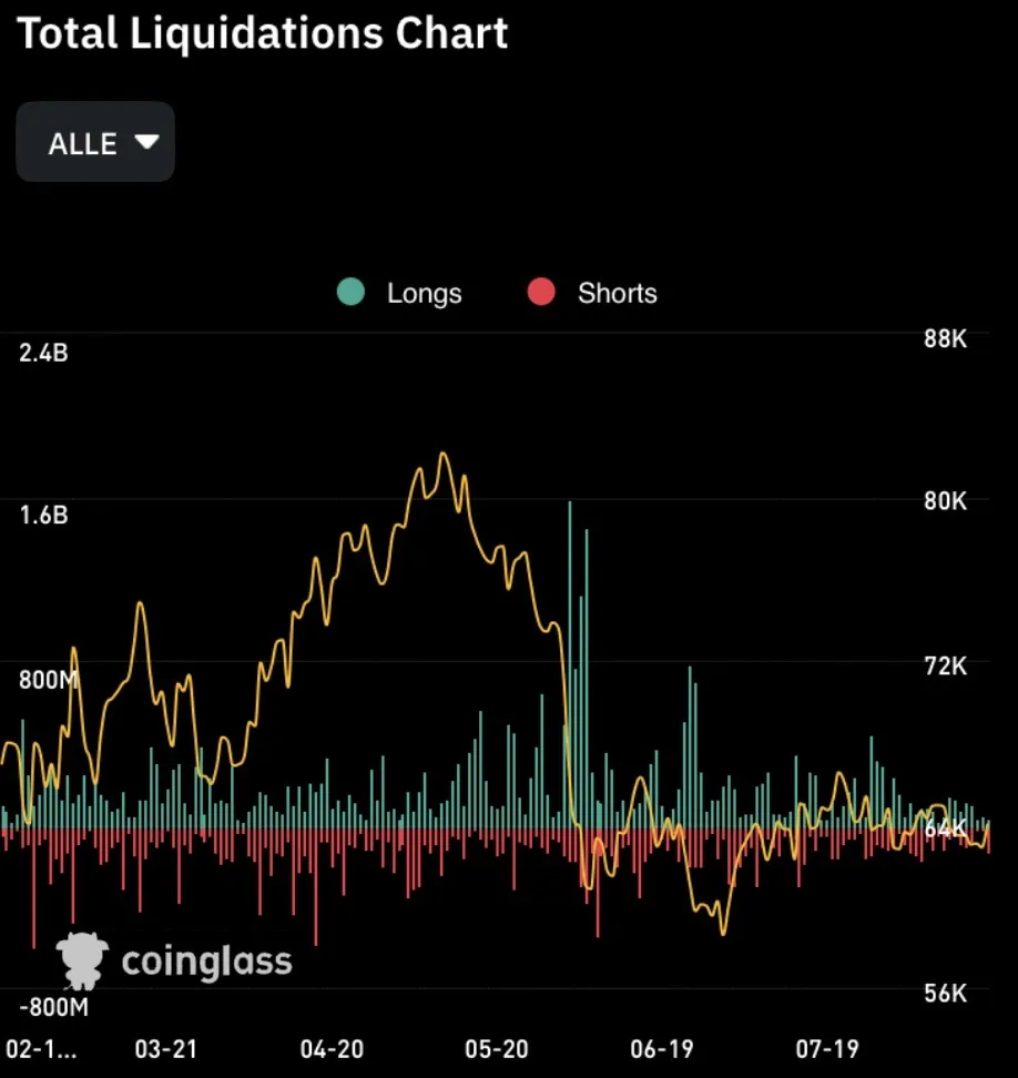
A perpetual futures contract, the dominant derivative structure in crypto trading, has no expiration date, and is kept tethered to the underlying spot price through the funding rate, a periodic payment exchanged directly between long and short position holders rather than through the roll mechanism described in Part VII. When the funding rate is positive, longs pay shorts, reflecting a market where leveraged positioning is skewed bullish; when it is negative, shorts pay longs, reflecting the opposite. Open interest is the aggregate value of outstanding leveraged positions across the market, a direct gauge of how much leverage is currently active. A liquidation cascade is the self-reinforcing mechanism behind crypto’s characteristically violent, fast moves: a sharp price swing forces the most highly leveraged positions to be closed involuntarily, and that forced closing itself adds further pressure in the same direction, triggering the next tier of leveraged positions to be liquidated in turn. The basis, the gap between the perpetual or futures price and the spot price, functions as a further real-time leverage and positioning gauge, extending the same concept already introduced generally in Part VII.

Custody and Technology Risk

Self-custody, holding assets in a wallet where the holder alone controls the private keys, commonly a cold wallet kept offline for security, gives complete control and removes any counterparty from the equation entirely, at the cost of complete personal responsibility: there is no recourse if a private key is lost. Exchange custody is more convenient and familiar but reintroduces exactly the kind of counterparty risk described for brokers in Part XVIII, the exchange itself becoming a single point of failure between the holder and their assets. Smart contract risk is the risk of a bug or an exploit in a protocol’s underlying code being used to drain funds, a technology-specific risk layer with no real equivalent in traditional finance. Bridge risk, already introduced above, and regulatory risk, the genuine, still-evolving and jurisdiction-dependent legal treatment of digital assets, round out a risk profile that is structurally different in kind, not merely in degree, from most of the traditional asset classes covered elsewhere in this guide.

Why Crypto Market Capitalisation Can Mislead

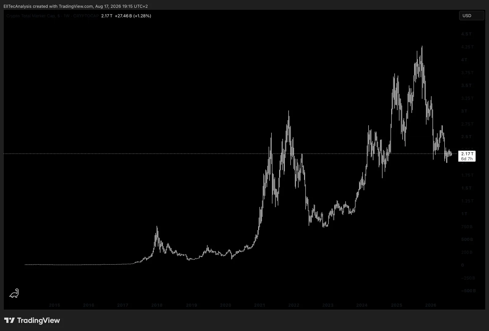
Market capitalisation is simply price multiplied by circulating supply, and for a thinly traded token, that headline figure can meaningfully overstate what could actually be realised by selling, since a comparatively small amount of actual selling can move the price of an illiquid token disproportionately, meaning the “value” implied by the last traded price was never genuinely available to every holder simultaneously. The FDV gap described above compounds this further: a token trading on a market cap calculated from a small circulating supply, with a large multiple of that supply still locked and scheduled to unlock over time, is arguably better compared against its FDV than its current market cap when judging genuine long-term valuation, since that is the supply base the token will eventually trade against.

Part XVI: Portfolio Construction, Position Sizing, and Risk Management

Diversification and risk management are not optional refinements layered onto a strategy after the fact. They are the strategy, in the sense that a portfolio’s survival through drawdowns determines whether it is ever around to benefit from a subsequent recovery.

Diversification

Diversification works by combining assets whose returns are not perfectly correlated, so that weakness in one part of a portfolio is offset, at least partially, by strength or stability elsewhere. It should operate across asset classes, not only within them: a portfolio holding twenty different technology stocks is not meaningfully diversified, because all twenty are exposed to the same sector-specific and rate-sensitivity risk. Genuine diversification spans equities, fixed income, commodities, and cash, and ideally spans geographies and currencies as well, precisely because correlations between asset classes shift and occasionally invert, exactly the regime-dependent behaviour covered in Part XIII’s intermarket analysis.

Portfolio Construction Approaches

Strategic asset allocation sets long-term target weights across asset classes based on an investor’s goals, horizon, and risk tolerance, and is meant to be held through ordinary market fluctuation rather than adjusted reactively. Tactical asset allocation deliberately deviates from those long-term targets for a defined period based on a specific market view, a shorter-horizon overlay on top of the strategic base. Core-satellite structures combine a large, low-cost, broadly diversified core holding, commonly built from the ETFs covered in Part VIII, with a smaller satellite sleeve of higher-conviction, more concentrated positions, giving a natural, structural home for single-name research such as EllTec’s own reports without exposing the entire portfolio to that concentrated risk. A barbell allocates capital to two extremes, very safe and very aggressive, deliberately avoiding the middle ground, on the logic that the safe portion protects against catastrophic loss while the aggressive portion captures outsized upside. Risk parity allocates capital so that each holding contributes roughly equal risk to the overall portfolio, rather than equal capital, which in practice means holding more of lower-volatility assets like bonds and less of higher-volatility assets like equities than a simple capital-weighted split would suggest. Minimum variance and maximum diversification are related optimisation approaches that construct a portfolio specifically to minimise overall volatility or maximise the diversification benefit across holdings, rather than targeting a specific return. Factor investing tilts a portfolio deliberately toward specific, historically rewarded characteristics, value, momentum, quality, and size being the most established, rather than toward market-cap weight alone. A concentrated portfolio, deliberately holding relatively few positions, trades away diversification for higher potential return if the specific theses are correct, at the direct cost of higher idiosyncratic risk if any one of them is not, the fundamental tradeoff every core-satellite structure is built to manage. Rebalancing periodically brings a portfolio’s actual weights back to their strategic targets, and portfolio drift, the gradual, unintentional deviation from those targets as different holdings perform differently over time, is exactly what rebalancing corrects for; done systematically, rebalancing also imposes a disciplined buy-low-sell-high mechanism, trimming what has outperformed and adding to what has lagged, without requiring any active market call at all. Cash and hedge allocations, deliberate, sized holdings of cash or explicitly protective positions, are themselves legitimate portfolio components with a defined purpose, not simply leftover, unallocated capital.

Quantitative Risk and Return Metrics

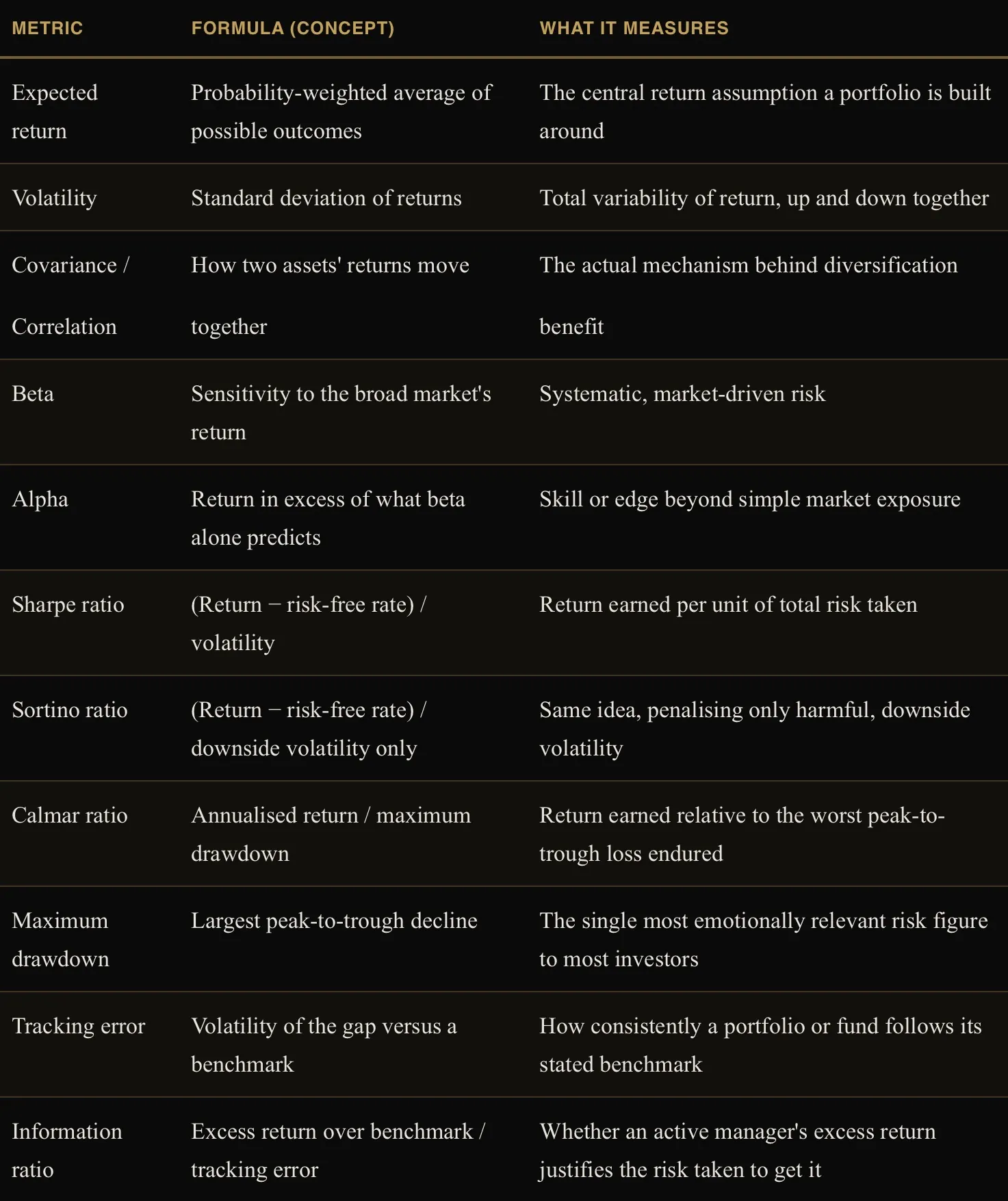
Sharpe and Sortino answer a similar question from a slightly different angle, and the difference matters: Sharpe penalises all volatility equally, including the upside surprises an investor is generally happy to receive, while Sortino penalises only downside volatility, which is why Sortino is often considered the more intuitively honest measure of risk actually experienced. Maximum drawdown, in practice, is frequently the risk statistic that determines whether an investor can actually stick with a strategy through a real drawdown or abandons it at the worst possible moment, making it arguably more behaviourally relevant than volatility itself.

Modern Portfolio Theory and the CAPM

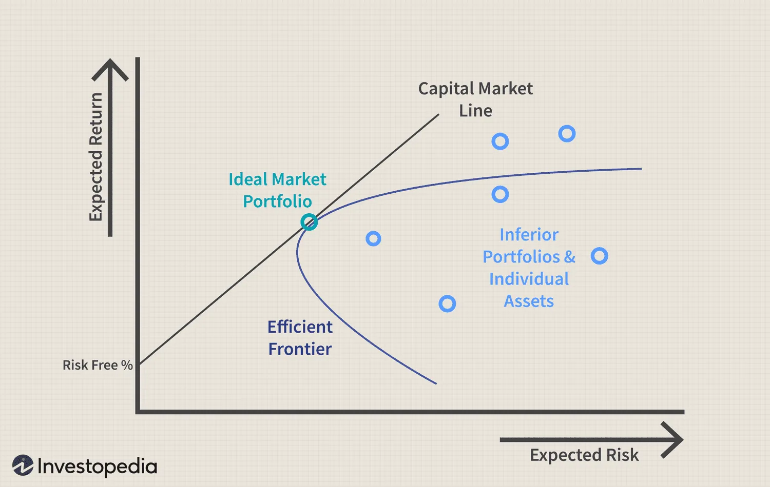
The metrics above did not emerge in isolation; they rest on a specific theoretical foundation built substantially by Harry Markowitz’s mean-variance framework. The core insight is that a rational investor should care about a portfolio’s overall risk and return together, not any single holding in isolation, and that combining imperfectly correlated assets can reduce a portfolio’s total volatility below what any individual holding carries on its own, the mathematical formalisation of the diversification benefit described throughout this guide. Plotting every possible combination of available assets by their expected return and volatility traces out the efficient frontier, the set of portfolios offering the highest possible expected return for each given level of risk; portfolios below that frontier are, by definition, suboptimal, since a better risk-return combination exists somewhere on the frontier itself. Adding a risk-free asset, cash or a government bill, to the mix produces the tangency portfolio, the single portfolio on the efficient frontier that, combined with varying amounts of the risk-free asset, produces the best possible risk-return tradeoff available at any risk level, and theoretically the portfolio every rational investor should hold in some proportion alongside cash. The Capital Asset Pricing Model, CAPM, builds directly on this framework to explain what return an asset should offer given its risk: expected return equals the risk-free rate plus that asset’s beta multiplied by the market risk premium, the same formula already used to estimate the cost of equity within the WACC calculation in Part V. Plotted across every level of beta, this relationship traces the Security Market Line, and an asset trading above that line is offering more return than its risk alone would justify, while one trading below it is offering less. In practice, CAPM’s single-factor, beta-only explanation of returns has proven incomplete, which is exactly what multi-factor models were built to address: the Fama-French framework extends CAPM with additional factors found to independently and persistently explain returns beyond market beta alone, size (smaller companies have historically outperformed larger ones on a risk-adjusted basis), value (cheap stocks have historically outperformed expensive ones, the empirical backbone behind the value investing strategy in Part IX), and profitability and investment (more profitable, more conservatively run companies have historically outperformed), with momentum, quality, and low-volatility factors added by later research as further, independently persistent return drivers, the same factors already introduced as factor investing earlier in this Part.

Tail Risk, VaR, and Expected Shortfall

The volatility measure used throughout this guide implicitly assumes returns are distributed in a reasonably well-behaved, bell-curve pattern, and real market returns are not: extreme moves, in both directions, happen considerably more often than a normal distribution would predict, a property known as fat tails. This matters directly for risk management, since a framework built entirely on standard deviation alone will systematically underestimate the odds and the severity of a genuine tail event, exactly the kind of event that produces the sharpest drawdowns and the liquidation cascades already covered in Part XVI. Value at Risk, VaR, is the standard institutional risk metric built to address this directly: it estimates the maximum expected loss over a given time horizon at a given confidence level, so a one-day 95% VaR of five percent means there is a 95% probability that losses over the next day will not exceed five percent of the portfolio. VaR’s own well-known limitation is that it says nothing about how bad the outcome could be within that remaining five percent of cases, the tail beyond the VaR threshold itself, which is exactly the gap Expected Shortfall, also called Conditional VaR or CVaR, is built to close: it measures the average loss specifically within that worst-case tail, rather than merely the threshold at its edge, giving a considerably more honest picture of genuine tail risk than VaR alone.

Position Sizing

Risk management begins with position sizing: no single position, however compelling the thesis, should be large enough that being wrong about it threatens the portfolio as a whole. Fixed-fractional sizing risks a constant, predefined percentage of total capital on any single position, commonly in the range of 0.5% to 2%, calculated as: risk budget (capital × risk percentage) divided by the per-share or per-unit distance between entry and stop, giving the position size directly. Volatility-based, or ATR-based, sizing uses the same formula but replaces a fixed percentage stop distance with a multiple of the Average True Range introduced in Part X, which automatically sizes positions smaller in more volatile assets and larger in calmer ones for the same underlying dollar risk. Portfolio heat is the aggregate risk currently at stake across every open position simultaneously; ten positions each individually risking two percent represents up to twenty percent of total capital at risk if every single one were to hit its stop at once, which is exactly why heat needs its own portfolio-level cap independent of the per-trade risk limit. Correlation-adjusted exposure addresses the same concern from a different angle: five positions that are all effectively long the same underlying macro factor, five different companies all highly sensitive to the same commodity price or the same interest-rate move, are not five independent risk budgets, they are closer to one large, concentrated one, however diversified they might look purely by ticker count. Leverage-adjusted exposure extends this further still: a leveraged position’s true size for risk-management purposes is its full notional exposure, not merely the smaller amount of capital actually committed as margin, exactly the distinction that makes the CFD and futures leverage covered in Parts IV and VII genuinely dangerous when sized only against posted margin rather than true exposure.

Risk of Ruin and the Kelly Criterion

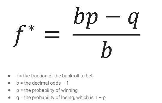
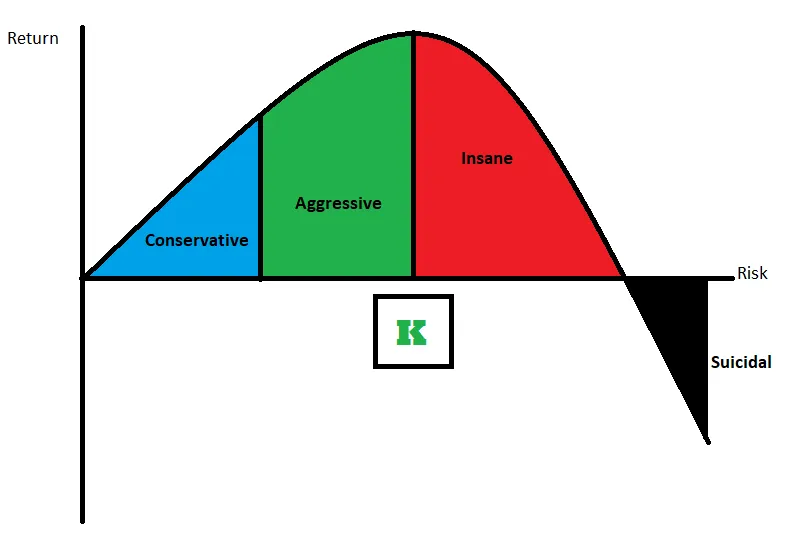
Risk of ruin is the mathematical probability that a given combination of position size, win rate, and payoff ratio eventually leads to a loss of capital severe enough to end the ability to keep trading at all, and it rises far faster than intuition suggests as risk per trade increases, which is the single strongest mathematical argument for disciplined, modest position sizing over any specific edge or forecast. The Kelly Criterion calculates the theoretically optimal fraction of capital to risk on a given bet, based on the edge (the probability of winning) and the odds (the payoff ratio if a win occurs); in practice, full Kelly sizing is considerably more aggressive, and more volatile, than most investors can tolerate, and it is highly sensitive to the accuracy of the win-rate and payoff estimates feeding into it, which is why practitioners overwhelmingly use a fraction of full Kelly, commonly half, deliberately trading some theoretical growth rate for a meaningfully smoother, more survivable equity curve.

Expected Value, Win Rate, and Why Position Sizing Beats a High Hit Rate

A trading or investing process can be reduced to a handful of simple statistics: win rate (the percentage of positions that are profitable), average win, average loss, the payoff ratio (average win divided by average loss), and the profit factor (total gross profit divided by total gross loss). Expected value per trade is simply (win rate × average win) minus (loss rate × average loss), and it is the number that actually determines long-run profitability, not the win rate in isolation. Consider two concrete examples. A trader who wins sixty percent of the time but lets losses run to twice the size of each win, and cuts winners early at half that size, has an expected value of (0.60 × 0.5R) − (0.40 × 2.0R) = 0.30R − 0.80R = −0.50R per trade, a losing process despite a majority-winning hit rate. A trader who wins only forty percent of the time but consistently lets winners run to twice the size of each loss, and cuts losses at a strict, predefined level, has an expected value of (0.40 × 2.0R) − (0.60 × 1.0R) = 0.80R − 0.60R = +0.20R per trade, a profitable process despite losing on the majority of individual trades. Risk management and position sizing, not the hit rate that feels most psychologically satisfying, is what actually separates these two outcomes.

The Psychology of Losing Money

Most investing mistakes are not analytical, they are psychological, and the same recurring biases show up across nearly every account that underperforms its own holdings.

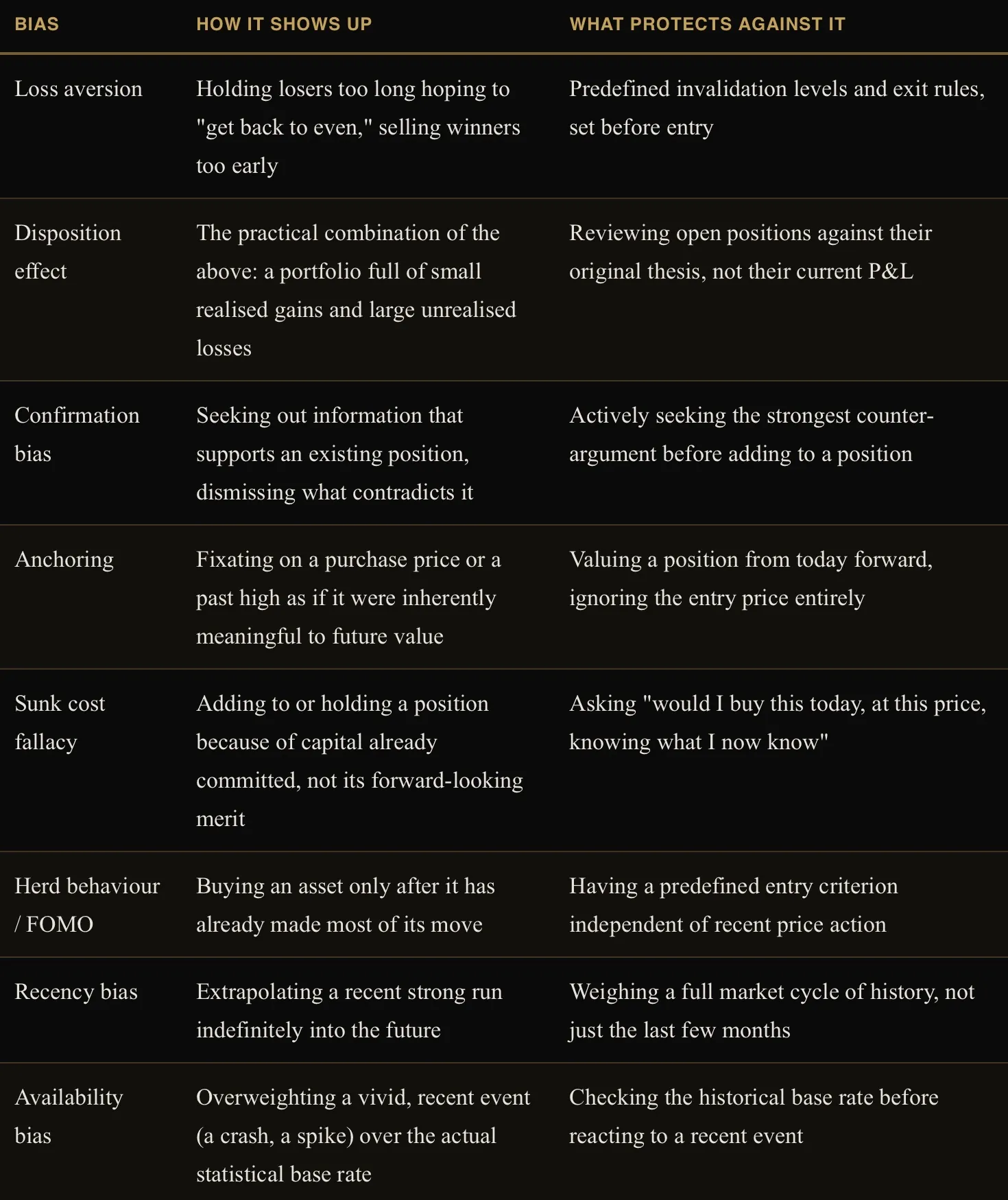
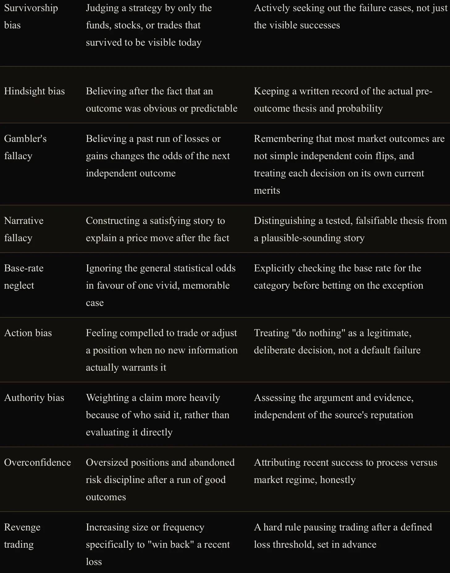
None of these biases are eliminated simply by knowing about them. They are managed by the same structural discipline this Part is built around: predefined position sizing, predefined invalidation levels, and a process that is followed regardless of how the investor currently feels about the position.

Part XVII: Broker, Custody, Regulation, and Tax

Broker Versus Exchange, and Where Assets Actually Sit

The broker-exchange-clearing-custodian distinction introduced in Part III becomes directly relevant here, since a retail investor’s actual protection in the event something goes wrong depends entirely on understanding which of these roles is failing. Segregated client assets is the regulatory requirement, standard across most developed markets, that client securities and cash are legally kept separate from the broker’s own balance sheet, meaning they are not available to the broker’s own creditors if the broker itself becomes insolvent. In practice, client assets are frequently pooled together in an omnibus account at the custodian level rather than titled individually to each client by name, which is normal and does not itself defeat the segregation protection, but it is worth understanding as the actual mechanical structure behind “my shares are held separately.” Investor compensation schemes exist in most jurisdictions as a further backstop specifically for cases where segregation itself fails, though the coverage limits, the assets covered, and the exact mechanics vary meaningfully by country and must be checked against the investor’s own jurisdiction and broker rather than assumed. It is worth stating the core distinction plainly, since the two are frequently conflated: a stock falling in value is market risk, an ordinary, expected feature of investing; a broker becoming insolvent and failing to return client assets is counterparty risk, a fundamentally different category of loss that segregation and compensation schemes exist specifically to address. A further distinction is worth holding onto for a bank, a broker, or a company alike: a liquidity crisis is being unable to access cash quickly enough to meet an immediate obligation despite the underlying assets being worth more than the liabilities, while a solvency crisis is the more serious condition where liabilities genuinely exceed assets regardless of timing. A fundamentally solvent institution can still fail purely from a liquidity crunch, a bank run being the textbook example, which is exactly why central banks maintain emergency lending facilities specifically to bridge liquidity gaps for otherwise solvent institutions, while a genuinely insolvent one cannot be rescued by liquidity alone, only by new capital or the restructuring process already described in Part II.

Rehypothecation and Execution Quality

Securities held in a margin account, as opposed to a standard cash account, are frequently subject to rehypothecation, the practice of the broker re-using client collateral for its own financing purposes, generally disclosed in the account agreement but rarely read closely, and it is a real, additional risk layer specific to leveraged and margin accounts rather than standard cash holdings. Best execution is the broker’s regulatory obligation to seek the best reasonably available outcome for a client’s order across price, speed, and likelihood of execution, and execution quality, how consistently a broker actually delivers on that obligation in practice, is worth genuine attention, since it directly affects realised returns in ways that are easy to overlook next to the more visible headline commission rate. The full, real cost of using a broker extends well beyond that headline commission: the bid-ask spread paid on every trade, FX conversion fees on any cross-currency transaction, financing or overnight fees on leveraged and margin positions, and inactivity fees charged on dormant accounts all add up, and a “commission-free” broker is never actually a fee-free one.

Regulatory Framework for European Retail Investors

MiFID II is the European Union’s core framework governing investor protection and market conduct across the bloc, setting the baseline rules brokers and product providers must follow. PRIIPs requires that packaged retail investment products, including many of the structured products covered in Part VII, carry a standardised Key Information Document, giving retail investors a consistent, comparable format for a product’s risk, cost, and potential outcome disclosure before they invest. UCITS, already introduced in Part VIII, is the specific regulatory wrapper most retail-marketed European funds and ETFs operate under. ESMA, the European Securities and Markets Authority, sets EU-wide product intervention measures, including the leverage restrictions on CFDs marketed to retail clients already flagged in Part IV, and BaFin is the German national regulator responsible for enforcing this framework domestically, with equivalent national regulators performing the same role across other EU member states. In the US, the SEC and FINRA perform broadly analogous functions, setting and enforcing securities market rules and broker conduct standards respectively. Two related but genuinely distinct investor-protection tests are worth knowing by name: suitability asks whether a specific product or strategy is appropriate for a specific investor’s actual circumstances, goals, and risk tolerance, while appropriateness asks the narrower question of whether that investor has sufficient knowledge and experience to understand the product’s risks at all, regardless of whether it suits their broader financial picture. Product intervention and leverage restriction powers, the ability of a regulator to directly restrict how a complex or high-risk product can be marketed to retail clients, are precisely why CFD leverage is capped for retail investors in the EU in the first place, closing the loop this guide opened without explanation back in Part IV.

Tax: A General, Non-Personalised Overview

Tax treatment of investments varies enormously by country and changes over time, and nothing in this section constitutes personalised tax advice; every reader should verify current rules with a qualified tax advisor familiar with their own specific jurisdiction before making any decision on this basis. With that said, a handful of concepts recur across most tax systems and are worth understanding in general terms. Capital gains, profit realised from selling an asset above its purchase price, are generally taxable, and many jurisdictions apply different rates depending on how long the asset was held before sale. Frequent realisation of gains carries a cost beyond the tax rate itself: tax drag is the compounding cost of paying tax along the way rather than deferring it, since every unit of currency paid in tax today is one that can no longer compound going forward, part of the structural, non-strategy-related case for the buy-and-hold approach introduced in Part IX, entirely independent of whether that approach also happens to pick better investments. Dividends are generally taxed as income, and are frequently subject to withholding tax deducted at source by the country where the underlying security is domiciled before the payment ever reaches the investor, with the rate sometimes reduced under a bilateral tax treaty between the investor’s home country and the source country, and in some cases partially reclaimable. Accumulating funds, introduced in Part VIII, reinvest income internally rather than distributing it as cash, and a meaningful number of jurisdictions still tax that internally reinvested income as if it had been received in cash, sometimes called phantom income, a detail worth checking specifically rather than assuming that “no cash received” means “nothing taxable.” ETF taxation more broadly depends heavily on both the fund’s own domicile and the investor’s tax residency, and the two can interact in ways that are genuinely not intuitive without checking the specific combination. Loss harvesting, deliberately realising a loss to offset a taxable gain elsewhere in the portfolio, is a widely used general technique, though a number of jurisdictions restrict the tax benefit if the same or a substantially identical security is repurchased within a short window afterward. Tax lots matter whenever an investor has purchased the same security at different times and different prices: which specific lot is deemed sold, commonly first-in-first-out by default or a specifically identified lot where the broker and jurisdiction allow it, directly changes the taxable gain or loss calculated on that sale. Some jurisdictions additionally levy a transaction tax or stamp duty on the trade itself, independent of whether it produced a gain or a loss. Brokers typically issue an annual tax statement summarising the year’s activity, but the legal responsibility for correct and complete tax reporting rests with the investor, not the broker, regardless of what that statement does or does not include.

Part XVIII: The Research Process and Decision Frameworks

Everything covered so far in this guide is a piece of vocabulary. This Part is where those pieces assemble into an actual, repeatable method, deliberately mirroring the structure every EllTec Analysis report is itself built around.

How to Analyse an Investment, Start to Finish

1. Understand the business

What does the company actually sell, to whom, and how does it make money, covered in Parts I and II.

2. Analyse the industry and competitive position

Who are the real competitors, is there a genuine moat, and how large is the addressable market, covered in Part V.

3. Analyse the macro environment

What phase of the cycle is the economy in, and is the policy and liquidity backdrop a tailwind or a headwind for this specific business, covered in Part XIII.

4. Analyse the financial statements

Work through the income statement, balance sheet, and cash flow statement directly rather than relying on someone else’s summary, covered in Part V.

5. Assess fundamental quality

Check earnings quality, leverage, and the specific red flags covered in Part V before trusting the headline numbers at face value.

6. Determine valuation

Build both a relative view, against peers and history, and where practical an absolute view, a DCF or a reverse DCF, covered in Parts V and VI.

7. Identify catalysts

What specific, datable events, an earnings report, a index rebalancing date, a scheduled central bank decision, could move the thesis forward, covered in Parts II and XIII.

8. Identify risks

What could go wrong that is specific to this business, this sector, and this macro backdrop, distinct from ordinary market risk.

9. Analyse the technical structure

What does the price structure and wave count actually show right now, covered in Parts X and XI.

10. Analyse sentiment and positioning

Is positioning already crowded in the direction of the thesis, or does room remain, covered in Part XII.

11. Build explicit bull, base, and bear scenarios

Not a single forecast, a probability-weighted range of outcomes, exactly the Alternative Scenarios structure used throughout EllTec’s own reports.

12. Define invalidation

The specific level or event that proves the thesis wrong, set before entry, not decided emotionally after the fact.

13. Determine position size

Using the frameworks in Part XVII, sized to the position’s specific risk, not to conviction alone.

14. Execute with the right instrument

Choose between the options covered in Parts IV and VII based on the view’s time horizon and risk tolerance, not habit.

15. Monitor the position

Track the specific catalysts and invalidation level identified in steps 7 and 12, not the position’s day-to-day price alone.

16. Reassess the thesis regularly

On a defined schedule or when genuinely new information arrives, distinct from reacting to every price fluctuation.

17. Define exit criteria in advance

Both the profit-taking framework and the loss-cutting framework should already exist before either is actually triggered.

Practical Decision Frameworks

Should I buy this stock?

Do I understand the business and how it makes money? Is the balance sheet and earnings quality sound (Part V)? Is the valuation reasonable relative to growth and peers? What does the technical structure suggest about timing (Parts X, XI)? What is the macro and sector backdrop (Part XIII)? What specifically would prove this thesis wrong? What position size keeps this from threatening the portfolio if it is (Part XVII)?

Is this stock actually cheap?

Cheap relative to what: its own history, its peers, or the market as a whole (Part V)? Is the low multiple explained by genuinely deteriorating fundamentals rather than genuine mispricing? What does PEG say once growth is accounted for? Would a reverse DCF’s implied growth rate look reasonable, or absurd?

Is this ETF suitable for long-term investing?

Broad and diversified, or thematic and concentrated (Part VIII)? Physical or synthetic replication, and is the resulting counterparty risk acceptable? What is the all-in cost, TER plus spread plus tracking difference, not the TER alone? Accumulating or distributing, and does that match the tax situation (Part XVIII)?

Is this bond attractive?

What is the yield to worst, not just the headline coupon (Part VI)? What does the credit rating say about default risk, and is the spread fair compensation for it? How does the duration exposure fit the current rate outlook (Part XIII)? Is there a genuinely more attractive risk-adjusted alternative at a similar duration and credit quality?

Should I use a stock, an ETF, an option, a CFD, or a certificate?

Direct ownership with no time limit and no leverage points toward a stock or ETF. A defined-risk, time-limited, leveraged view points toward an option. A short-term, tactical view where issuer and counterparty risk are genuinely understood and accepted points toward a CFD or certificate (Part VII). Income generation against an existing holding points toward a covered call. The instrument should always be chosen to match the view’s actual time horizon and risk tolerance, never the reverse.

How much should I invest in this specific idea?

What is the position’s defined risk, from entry to stop? What percentage of total capital am I willing to risk on this one idea? What does that make the resulting position size, and does that size still fit within current total portfolio heat (Part XVII)? Is this position genuinely independent of other existing holdings, or correlated with them?

Is the current market risk-on or risk-off?

What are credit spreads doing, widening or narrowing (Part XII)? Where does the VIX sit, and what is its trend? What is the yield curve and real yields doing (Part XIII)? Is sector leadership cyclical or defensive right now? Is the dollar strengthening or weakening (Parts XIII, XIV)?

Is this a fundamental problem or merely a technical correction?

Has anything actually changed in the business, its earnings, or its guidance (Parts II, V)? Or is this move consistent with a corrective wave within an otherwise intact structure (Part XI)? Has the invalidation level actually been breached, or only approached? Does volume and sentiment behaviour suggest exhaustion of a correction, or genuine, sustained distribution (Parts X, XII)?

Should I cut the position?

Has the original invalidation level actually been hit? If so, cut. Has genuinely new information changed the thesis, independent of price action alone? If so, reassess honestly. Am I considering holding purely to avoid realising a loss? If so, that is loss aversion (Part XVII), not analysis. Does the position still fit within current portfolio heat and correlation exposure regardless of its own individual merit?

Part XIX: Common Retail Investor Mistakes

Most of what follows has already been explained in full elsewhere in this guide; what is collected here is the practical, memorable list of how those concepts actually go wrong in practice.

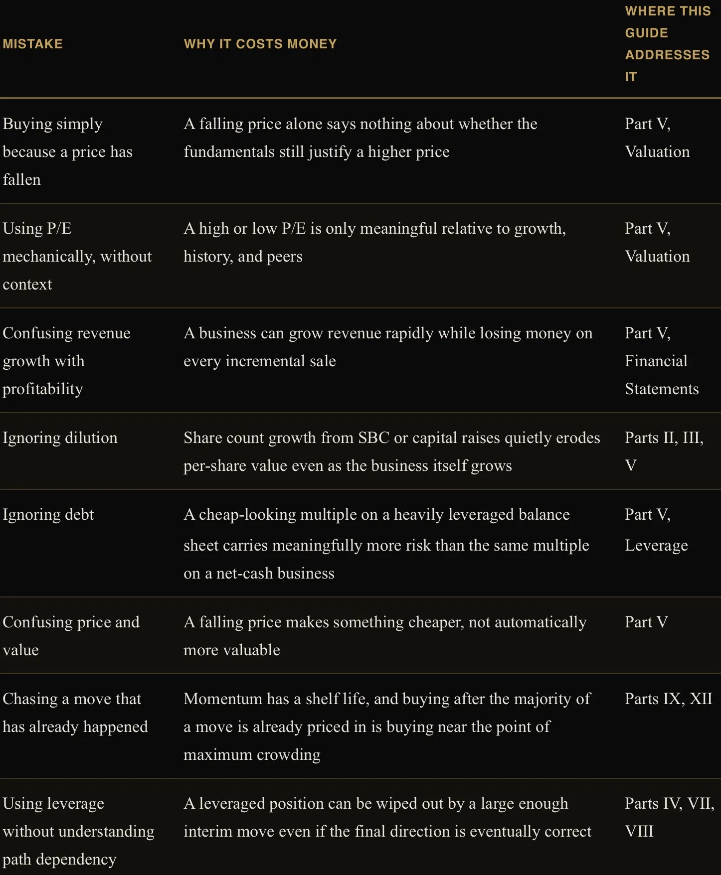
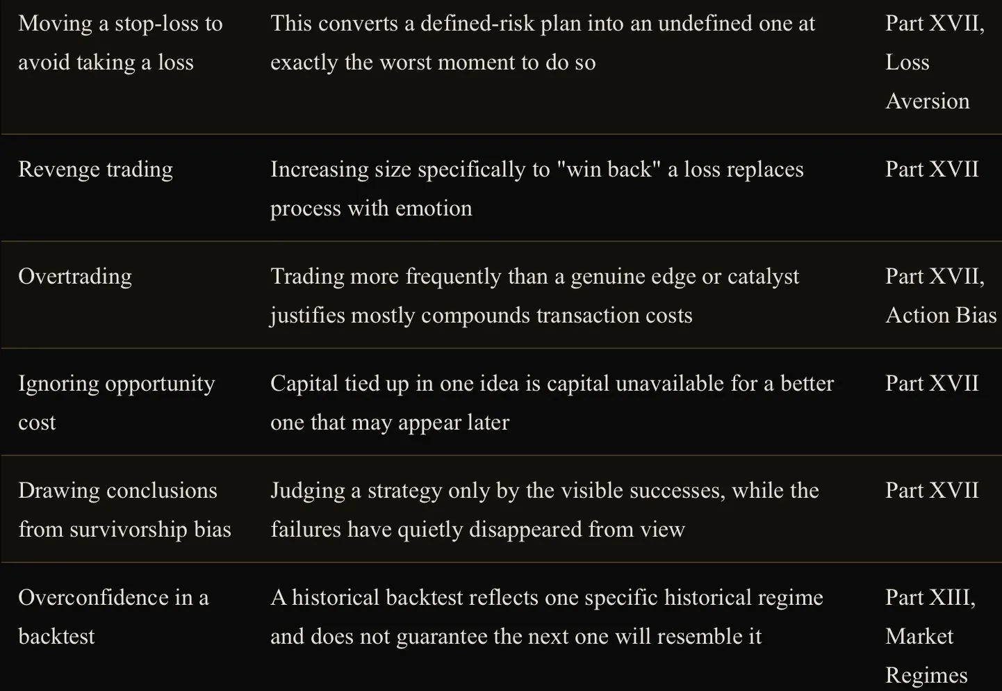
Part XX: Why EllTec Analysis Builds Research This Way

There are broadly two failure modes in the research that gets published for retail investors. The first is pure technical analysis delivered as a signal without context: a chart with an arrow on it and no explanation of the macro or fundamental backdrop the position is operating within, and critically, no defined level at which the idea is wrong. The second is pure fundamental research delivered without any timing framework at all: a well-argued thesis on why a company is undervalued, with no structure for when or how to actually enter, scale, or exit a position, and no acknowledgement that a correct long-term thesis can still produce years of underperformance if entered at the wrong point in the cycle.

EllTec Analysis is built to sit between those two failure modes rather than to choose one of them. Every report combines a top-down macro and fundamental read, valuation, profitability, margins, balance sheet strength, and the broader correlation and macro backdrop the asset operates within, with a bottom-up Elliott Wave and Fibonacci technical structure that translates that fundamental view into an actual, tradeable framework: defined target zones, defined alternative scenarios with their own trigger levels, and a defined invalidation point at which the primary structural interpretation is proven wrong.

This is deliberately a scenario-based approach rather than a single-point prediction. Markets are probabilistic, not deterministic, and a research process that presents one confident price target with no acknowledgement of what would prove it wrong is presenting false certainty. Structuring alternative scenarios alongside the primary count, and stating plainly whether the fundamental backdrop supports or complicates each of them, is what allows a reader to actually manage risk around the idea rather than simply hoping the first scenario plays out.

That is also, ultimately, the purpose behind every EllTec Analysis report: not to hand a reader a prediction to follow blindly, but to hand them a structure clear enough that they can evaluate it, disagree with parts of it, and make their own informed decision with defined risk on either side of the trade. Market structure clearly explained is not a slogan. It is the actual design principle behind every report this publication produces, and it is the same principle this entire guide has been built around, from the first page to the last.

Conclusion

Financial markets reward process far more reliably than they reward prediction. An investor who understands what asset class they are actually holding, what corporate events and mechanics move an individual stock, how a trade actually moves through the market’s plumbing, how to read a company’s own financial statements and value it honestly, what instrument they are holding a position through, what strategy that position is supposed to serve, what the full technical and macroeconomic toolkit is currently signalling, and how to size and manage the risk of every position in a portfolio, is an investor equipped to make genuinely informed decisions rather than reactive ones.

None of this removes uncertainty from markets, and nothing in this guide should be read as a guarantee of any outcome. Every framework covered here, from a DCF model to an Elliott Wave count to a position-sizing formula, produces a probability-weighted view of the future, not a certainty. What this guide provides instead is something more durable than a single correct forecast: a complete, coherent framework sturdy enough to hold up when markets get difficult, extensive enough to serve as a genuine standing reference rather than a one-time read, and honest enough to name its own limits along the way. That is exactly when a framework is needed most, and it is exactly what this guide, and every report EllTec Analysis publishes, is built to provide.

Glossary

An alphabetical reference to the technical terms introduced throughout this guide. Each entry points back to the Part where the concept is explained in full.

A

Accrued interest. Interest earned on a bond since its last coupon payment, added to the clean price to arrive at the dirty price actually paid (Part VI).

ADR / GDR. American/Global Depositary Receipt, a domestically-listed certificate representing shares of a foreign company, held in custody by a depositary bank (Part III).

Activist investor. A fund that accumulates a stake specifically to push for operational, strategic, or board-level change (Part II).

Alpha. Return earned in excess of what an asset’s beta alone would predict, a rough measure of skill beyond market exposure (Part XVII).

Advance/Decline Line. A cumulative running total of advancing minus declining stocks within an index, used to check whether a market move is broad-based (Part X).

Alternation. The Elliott Wave guideline that waves 2 and 4 within an impulse tend to differ from each other in form and complexity (Part XI).

American option. An option that can be exercised at any point up to expiration, as opposed to European style (Part VII).

Amortisation. Spreading the cost of an intangible asset over its useful life (Part V).

Anchoring. The bias of fixating on a reference price, such as a purchase price, as if it were inherently meaningful to future value (Part XVII).

Assignment. The obligation triggered for an option seller when the buyer exercises their right (Part VII).

AUM. Assets Under Management, the total value of assets a fund holds, a proxy for its liquidity and closure risk (Part VIII).

Authorised Participant. The institutional firm that creates and redeems ETF shares directly with the fund, keeping market price tethered to NAV (Part VIII).

B

Backwardation. A futures curve where futures prices sit below the spot price, often reflecting near-term supply tightness (Parts VII, XV).

Balance sheet. The financial statement showing what a company owns and owes at a single point in time (Part V).

Basis. The gap between a futures or perpetual price and the underlying spot price (Parts VII, XVI).

Beta. An asset’s sensitivity to the broad market’s return (Part XVII).

Bid-ask spread. The gap between the best available buy and sell price, the implicit cost of trading immediately (Part III).

Bonus certificate. A structured product paying a defined bonus at maturity provided the underlying never touches a lower barrier (Part VII).

Breakeven inflation. The market-implied inflation expectation, derived from the gap between a nominal bond’s yield and an equivalent inflation-linked bond’s yield (Part XIII).

Bridge (crypto). Infrastructure connecting separate blockchains, allowing assets to move between them, a distinct and historically significant risk category (Part XVI).

Bull/bear steepener/flattener. The four ways a yield curve’s shape can shift, depending on whether short or long yields move by more (Part VI).

Business cycle. The recurring sequence of expansion, peak, contraction, and trough that economies move through (Part XIII).

Buyback. See Share buyback.

C

Calendar effect. A statistically recurring seasonal return pattern, such as turn-of-month strength, with no clear fundamental cause (Part IX).

Calendar spread. An options strategy combining a short near-term option and a long longer-term option at the same strike (Part VII).

Capital allocation. How management deploys the cash a business generates across reinvestment, acquisitions, debt paydown, dividends, and buybacks (Part V).

Cap rate (capitalisation rate). A property’s Net Operating Income divided by its market value, real estate’s rough equivalent of an earnings yield (Part I).

Carry trade. Borrowing in a low-yielding currency to invest in a higher-yielding one, earning the rate differential (Part XIV).

Cash conversion. Operating cash flow divided by net income, a check on whether reported profit is translating into actual cash (Part V).

CDS (Credit Default Swap). A derivative functioning as insurance against an issuer’s default (Part VI).

Certificate of deposit. A bank time deposit paying a fixed rate for a fixed term (Part VI).

Circuit breaker. A market-wide mechanism automatically pausing trading after a large index decline within a session (Part III).

Clean price. A bond’s quoted price excluding accrued interest (Part VI).

Clearing house. The intermediary that becomes the counterparty to both sides of a trade, removing bilateral counterparty risk (Part III).

Commercial paper. Short-term unsecured corporate debt used to fund immediate working capital needs (Part VI).

Common shares. Equity carrying voting rights and a variable, residual claim on earnings (Part III).

Confirmation bias. Seeking and overweighting information that supports an existing position while dismissing what contradicts it (Part XVII).

Contango. A futures curve where futures prices sit above the spot price, often reflecting storage and financing costs (Parts VII, XV).

Convenience yield. The benefit of holding a physical commodity now rather than a future claim on it, especially valuable when supply is tight (Part XV).

Convertible bond. A bond giving the holder the option to convert into a set number of shares (Parts II, VI).

Convexity. The correction to duration’s linear price-yield estimate, capturing the curvature in that relationship (Part VI).

Core-satellite. A portfolio structure combining a low-cost diversified core with a smaller, higher-conviction satellite sleeve (Part XVII).

Correlation. How closely two assets’ returns move together, on a scale from minus one to plus one, and a value that shifts across market regimes (Part XIII).

Cost of carry. The financing plus storage cost of holding an asset until delivery, minus any income earned, the theoretical driver of a futures curve’s shape (Part VII).

Corrective wave. A three-wave, or complex, price structure moving against the larger trend (Part XI).

COT report. The CFTC’s weekly breakdown of positioning by participant type in US futures markets (Part XII).

Coupon. A bond’s stated annual interest payment (Part VI).

Covered call. Selling a call option against an existing stock holding to generate income (Part VII).

Credit rating. An assessment by Moody’s, S&P Global, or Fitch of an issuer’s creditworthiness, running from AAA down through speculative grade (Part VI).

Credit spread. The extra yield investors demand to hold corporate debt over comparable government debt, and a leading cross-asset stress gauge at the market-wide level (Parts VI, XII).

CTA (Commodity Trading Advisor). A fund running largely systematic, trend-following strategies across futures markets (Part XII).

Current ratio. Current assets divided by current liabilities, a short-term liquidity measure (Part V).

Current yield. A bond’s coupon divided by its current price (Part VI).

D

Dark pool. A private trading venue where orders are matched without displaying order interest publicly beforehand, used mainly for large institutional orders (Part III).

Days to cover. Short interest expressed as a multiple of average daily trading volume (Parts IV, XII).

DCF (Discounted Cash Flow). A valuation method estimating value from projected future cash flows discounted back to the present (Part V).

Dealer gamma / GEX. The aggregate directional hedging pressure created by market makers’ own options books, which can dampen or amplify volatility depending on its sign (Part XII).

Declaration date. The date a company’s board formally announces a dividend (Part II).

Deferred revenue. Cash already collected for a service not yet delivered, recorded as a liability (Part V).

Delisting. Removal of a company’s shares from an exchange, voluntary or involuntary (Part II).

Delta. An option’s sensitivity to a $1 move in the underlying (Part VII).

Diagonal (Elliott Wave). A wedge-shaped motive wave variant appearing at the start or end of a larger trend (Part XI).

Dilution. Any increase in shares outstanding that reduces each existing shareholder’s proportional ownership (Parts II, III).

Dirty price. A bond’s actual settlement price, including accrued interest (Part VI).

Discount certificate. A structured product purchased below the underlying’s price in exchange for a capped payout (Part VII).

Disinflation. Inflation that remains positive but is decelerating, distinct from deflation (Part XIII).

Diversification. Combining assets whose returns are not perfectly correlated to reduce overall portfolio risk (Part XVII).

Dividend. A portion of company profit distributed directly to shareholders (Part II).

DRIP. Dividend Reinvestment Plan, automatically using dividend cash to purchase additional shares (Part II).

Duration. A bond’s price sensitivity to a change in interest rates, expressed as an approximate percentage move per 1% yield change (Part VI).

DXY. The US Dollar Index, measuring the dollar against a basket of major currencies (Parts XIII, XIV).

E

Earnings call. The scheduled conference call following an earnings release where management discusses results with analysts (Part II).

Earnings yield. EPS divided by price, the inverse of P/E, used to compare equities against bond yields (Part V).

EBIT. Earnings before interest and tax, operating income (Part V).

EBITDA. EBIT plus depreciation and amortisation, a proxy for pre-capex cash generation (Part V).

ESG. Environmental, Social, and Governance, a scoring framework applied alongside or instead of traditional fundamentals, with no single agreed methodology across rating providers (Part V).

Efficient frontier. The set of portfolios offering the highest possible expected return for each given level of risk (Part XVII).

Efficient Market Hypothesis (EMH). The theory that asset prices already reflect available information, in weak, semi-strong, and strong forms (Part IX).

Expected Shortfall / CVaR. The average loss within the worst-case tail beyond the VaR threshold (Part XVII).

EPS. Earnings per share, net income divided by shares outstanding (Part V).

Equity risk premium. The excess return equities are expected to deliver over a risk-free bond (Part V).

ESMA. The European Securities and Markets Authority, which sets EU-wide product intervention measures (Part XVIII).

ETC / ETN / ETP. Exchange-Traded Commodity, Note, and the broader Product category, unsecured issuer debt tracking an index or commodity, distinct from an ETF’s fund structure (Part VII).

EV (Enterprise Value). Market capitalisation plus total debt minus cash, the cost of acquiring an entire business (Part V).

Ex-dividend date. The date on or after which a buyer is no longer entitled to an upcoming dividend (Part II).

Exercise. An option buyer’s act of using their right to buy or sell at the strike (Part VII).

Expected value. Win rate multiplied by average win, minus loss rate multiplied by average loss, the figure that actually determines long-run profitability (Part XVII).

Expiration. The date an option or futures contract ceases to exist (Part VII).

Extension (Elliott Wave). One of the three motive sub-waves becoming disproportionately larger than the other two (Part XI).

Extrinsic value. The portion of an option’s premium beyond its intrinsic value, driven by time and implied volatility (Part VII).

F

Factor certificate. A structured product targeting a fixed daily leverage multiple, subject to volatility decay (Part VII).

Fama-French factors. A multi-factor extension of CAPM adding size, value, profitability, and investment as independent return drivers (Part XVII).

Fat tails. The tendency of real market returns to produce extreme moves more often than a normal distribution predicts (Part XVII).

FCF (Free Cash Flow). Operating cash flow minus capital expenditure, the cash genuinely available to shareholders and creditors (Part V).

FCF yield. Free cash flow divided by market cap or enterprise value (Part V).

Fed Funds rate. The US central bank’s own overnight policy rate (Part VI).

Financial conditions. A composite gauge combining rates, credit spreads, equity volatility, and the dollar into a single measure of looseness or tightness (Part XIII).

Fixed-fractional sizing. Risking a constant percentage of capital on any single position (Part XVII).

Flat (Elliott Wave). A sideways 3-3-5 corrective structure (Part XI).

Floating-rate bond. A bond whose coupon resets periodically against a reference rate (Part VI).

Forward contract. An OTC agreement to buy or sell an asset at a set price on a future date, carrying counterparty risk a futures contract does not (Part VII).

Forward guidance. A central bank’s communication about its likely future policy path (Part XIII).

Free float. Shares actually available for public trading, excluding insider, strategic, or locked-up holdings (Part III).

Funding rate. The periodic payment exchanged between long and short holders of a perpetual futures contract to keep it tethered to spot (Parts XII, XVI).

G

Gamma. Sensitivity of an option’s Delta itself to a $1 move in the underlying (Part VII).

Gap. Price opening away from the prior session’s close (Parts II, X).

Green bond. A debt instrument where proceeds are contractually earmarked for environmentally beneficial projects (Part V).

Greenwashing. A fund or company overstating its genuine environmental or social credentials relative to its actual practices (Part V).

Goodwill. The premium paid in an acquisition above the fair value of a target’s identifiable net assets (Part V).

GTC (Good-Till-Cancelled). An order that remains active until filled or manually withdrawn (Part IV).

Guidance. Management’s forward-looking outlook for a coming period (Part II).

H

Herd behaviour. Piling into an asset only after it has already made most of its move (Part XVII).

High yield. Corporate debt rated below investment grade, also called junk (Part VI).

Hindsight bias. Believing after the fact that an outcome was obvious or predictable (Part XVII).

I

Impairment. A write-down taken when an asset, often goodwill, is no longer worth what was paid for it (Part V).

Implied volatility. The market’s forward-looking volatility estimate, backed out of an option’s price (Part VII).

Impulse. The textbook five-wave motive structure in Elliott Wave (Part XI).

Income statement. The financial statement showing whether a business made money over a period (Part V).

Index rebalancing. Periodic adjustment of an index’s constituent weights to match its methodology (Part II).

Initial margin. The deposit required to open a futures position (Part VII).

Insider transaction. Buying or selling by a company’s own executives and directors in its own shares (Part II).

Interest coverage. EBIT divided by interest expense, the cushion above the obligation to service debt (Part V).

Intrinsic value (option). The amount by which an option is currently in-the-money (Part VII).

Invalidation. The specific price level or event beyond which a technical or fundamental thesis is proven wrong (Parts V, XI, XVII).

Investment grade. Corporate or sovereign debt rated BBB-/Baa3 or above (Part VI).

IPO. Initial Public Offering, a company selling shares to the public for the first time (Part II).

ITM / ATM / OTM. In-the-money, at-the-money, and out-of-the-money, describing an option’s moneyness (Part VII).

IV rank / percentile. A stock’s current implied volatility contextualised against its own recent history (Part VII).

K

Kelly Criterion. A formula for the theoretically optimal fraction of capital to risk on a given bet, given edge and odds (Part XVII).

Knock-out certificate. A structured product automatically terminated if the underlying touches a defined barrier (Part VII).

L

Lagging indicator. A tool or data release that confirms a move or trend only after it has already happened (Parts X, XIII).

Leading indicator. A tool or data release that attempts to anticipate a move or trend before it fully develops (Parts X, XIII).

Leverage. Using borrowed capital or derivative structures to amplify exposure beyond capital committed (Parts IV, VII, XVII).

Liquidation cascade. A self-reinforcing unwind where a price move forces leveraged positions closed, adding further pressure in the same direction (Part XVI).

Liquidity crisis / Solvency crisis. Being unable to access cash for an immediate obligation despite sufficient assets, versus liabilities genuinely exceeding assets (Part XVIII).

Liquidity heatmap. A visualisation of resting order concentration across price levels in an order book (Part X).

Lock-up period. The contractual window after an IPO during which insiders cannot sell their shares (Part II).

Loss aversion. Feeling the pain of a loss more intensely than the pleasure of an equivalent gain (Part XVII).

M

M2. A broad measure of money supply, watched as a gauge of aggregate system liquidity (Part XIII).

Macaulay duration. The time-weighted average of when a bond’s cash flows are received, the basis for modified duration (Part VI).

Maintenance margin. The minimum account balance that must be sustained on a futures or margin position after it is opened (Parts IV, VII).

Margin call. A demand for additional funds when an account falls below required maintenance margin, often forcing liquidation (Part IV).

Margin debt. The aggregate level of leverage investors are carrying against their portfolios, a structural risk gauge (Part XII).

Market depth. The amount of order size resting at each price level in the order book (Part III).

Market impact. The price move caused by a trade itself when its size is large relative to available liquidity (Part III).

Market maker. An entity continuously quoting both a bid and an ask, providing liquidity (Part III).

Market order. An order that executes immediately at the best currently available price (Part IV).

Mean reversion. A strategy based on prices snapping back toward a statistical or technical baseline (Part IX).

Merger. Two companies combining into one (Part II).

MiFID II. The EU’s core investor-protection and market-conduct framework (Part XVIII).

Modified duration. The practical, price-sensitivity version of duration derived from Macaulay duration (Part VI).

Market Breadth. How many individual constituents of an index are actually participating in a move, distinct from the index level alone (Part X).

McClellan Oscillator. A smoothed momentum measure derived directly from advance/decline data (Part X).

Momentum. The tendency for strong recent performance to persist over intermediate horizons (Part IX).

Moneyness. The relationship between an option’s strike and the current underlying price (Part VII).

Money market fund. A pooled vehicle holding short-term, highly liquid instruments (Part VI).

Motive wave. A five-wave Elliott Wave structure moving in the direction of the larger trend (Part XI).

Moving average. A smoothed average price over a lookback period, used as a trend filter and dynamic support/resistance (Part X).

Multiple expansion/contraction. A rising or falling valuation multiple, which can drive return independently of earnings growth (Part V).

Mutual fund. An actively or passively managed pooled vehicle priced once daily (Part IV).

N

New Highs / New Lows. The count of index constituents hitting a fresh 52-week high or low in a session, a breadth read on narrowing or broadening leadership (Part X).

NAV (Net Asset Value). The per-share value of a fund’s actual underlying holdings (Part VIII).

Net Debt/EBITDA. Net debt divided by EBITDA, the years of current cash generation needed to repay net debt (Part V).

NOI (Net Operating Income). A property’s rental income minus operating expenses, before financing costs and taxes (Part I).

Net margin. Net income divided by revenue (Part V).

O

OAS (Option-Adjusted Spread). The extra yield a bond offers over a government benchmark after adjusting for embedded options (Part VI).

OCO (One-Cancels-the-Other). An order pairing a profit target and a stop-loss so that executing either cancels the other (Part IV).

Omnibus account. A pooled account structure where client assets are held together rather than individually titled (Part XVIII).

Open interest. The aggregate value of outstanding leveraged positions in a derivative market (Parts XII, XVI).

Operating leverage. How a company’s fixed-versus-variable cost structure amplifies profit swings relative to revenue swings (Part V).

Operating margin. Operating income (EBIT) divided by revenue (Part V).

Order book. The real-time, price-ranked list of resting buy and sell orders (Part III).

OIS (Overnight Index Swap). A derivative rate based on expected average overnight rates, used as a cleaner benchmark than term rates (Part VI).

P

Payment date. The date a declared dividend is actually paid (Part II).

Payment for order flow. An arrangement where market makers pay brokers for the right to execute retail order flow directly (Part III).

Payoff ratio. Average win divided by average loss (Part XVII).

PEG ratio. Forward P/E divided by expected EPS growth (Part V).

Perpetual futures. A futures contract with no expiration, tethered to spot via the funding rate (Part XVI).

PPP (Purchasing Power Parity). The theory that exchange rates should adjust to equalise the price of an identical basket of goods across countries (Part XIV).

Preferred shares. Equity with a fixed dividend priority over common shares but usually no voting rights (Part III).

Premium/discount to NAV. The gap between an ETF’s market price and its underlying NAV (Part VIII).

Price discovery. The continuous process by which order flow arrives at a market-clearing price (Part III).

PRIIPs. The EU requirement that packaged retail investment products carry a standardised Key Information Document (Part XVIII).

Private credit. Loans originated directly by non-bank lenders to companies not efficiently served by banks or the public bond market (Part I).

Private equity. Funds that acquire established private companies, or take public companies private, to improve and later exit them (Part I).

Private placement. Selling new shares or debt directly to a small number of institutional investors outside the public market (Part II).

Proof of Stake. A consensus mechanism where validators lock up tokens as collateral to secure a network (Part I).

Proof of Work. A consensus mechanism where miners solve computationally expensive puzzles to secure a network (Part I).

Protective put. Buying a put against an existing stock holding as downside insurance (Part VII).

Proxy fight. The mechanism by which an activist investor solicits shareholder votes against management’s recommendation (Part II).

Put-call parity. The no-arbitrage relationship linking a call price, a put price, and the underlying at the same strike and expiry (Part VII).

Q

QE (Quantitative Easing). Central bank purchases of bonds to inject liquidity and hold longer-term yields down (Part XIII).

QT (Quantitative Tightening). The reverse of QE, allowing a central bank’s balance sheet to shrink (Part XIII).

Quick ratio. Current assets minus inventory, divided by current liabilities, a stricter liquidity test (Part V).

R

Real yield. A bond’s yield minus expected inflation (Parts VI, XIII).

Robo-Advisor. An automated portfolio management service building and rebalancing a diversified portfolio based on a stated risk profile (Part IV).

Record date. The date a company checks its books to determine who is owed a declared dividend (Part II).

Recovery value. What bondholders actually receive if an issuer defaults (Part VI).

Reflation. A deliberate, policy-driven effort to push growth and inflation back up from a depressed level (Part XIII).

Rehypothecation. A broker re-using client collateral, typically from a margin account, for its own purposes (Part XVIII).

Repo market. Where institutions borrow cash short-term against high-quality collateral (Part VI).

Reverse convertible. A structured product paying an enhanced coupon in exchange for bearing downside risk below a defined level (Part VII).

Reverse DCF. Solving for the growth rate a current market price already implies (Part V).

Reverse split. A stock split that consolidates shares to raise the nominal price (Part II).

Rho. An option’s sensitivity to a change in interest rates (Part VII).

Rights offering. Giving existing shareholders the right to buy additional shares, usually at a discount (Part II).

Risk of ruin. The mathematical probability that a given risk approach eventually leads to catastrophic capital loss (Part XVII).

Risk parity. Allocating capital so each holding contributes roughly equal risk, rather than equal capital (Part XVII).

ROA. Return on Assets, net income divided by total assets (Part V).

ROCE. Return on Capital Employed, EBIT divided by capital employed (Part V).

ROE. Return on Equity, net income divided by shareholders’ equity (Part V).

ROIC. Return on Invested Capital, a capital-structure-neutral profitability measure (Part V).

Roll yield. The return earned specifically from rolling an expiring futures contract into the next one (Parts VII, XV).

S

Sampling. An ETF replication method holding a representative subset of an index’s constituents (Part VIII).

Security Market Line. The CAPM relationship plotting expected return against beta (Part XVII).

Swap. An agreement to exchange one stream of cash flows for another; interest rate, FX, and Total Return Swaps are the most common institutional forms (Part VII).

Securities lending. Lending out held securities, by a broker or a fund, in exchange for a fee (Parts III, VIII).

Settlement. The legal transfer of ownership and cash after a trade, occurring on the settlement date (Part III).

Share buyback. A company repurchasing its own stock on the open market (Part II).

Short interest. The percentage of a stock’s available float currently sold short (Parts IV, XII).

Short selling. Selling a borrowed asset with the intent to buy it back later at a lower price (Part IV).

Short squeeze. A rapid, self-reinforcing price spike forcing short sellers to buy back at a loss (Part IV).

Sharpe ratio. Return in excess of the risk-free rate, divided by total volatility (Part XVII).

Slippage. The gap between an order’s expected and actual execution price (Part III).

SOFR. The Secured Overnight Financing Rate, the primary US short-term benchmark rate (Part VI).

Sortino ratio. Like the Sharpe ratio, but penalising only downside volatility (Part XVII).

SPAC. A shell company that lists publicly to later merge with a private operating company (Part II).

Special dividend. A one-off dividend outside a company’s regular schedule (Part II).

Spin-off. Separating an existing division into its own independently listed company (Part II).

Spread duration. Sensitivity specifically to a change in credit spread, rather than the risk-free rate (Part VI).

Stablecoin. A cryptocurrency pegged to a reference asset, almost always the US dollar (Part I).

Stagflation. High inflation combined with stagnant growth and elevated unemployment (Part XIII).

Stock-based compensation. Equity paid to employees and executives, a real economic cost and dilution source (Parts II, V).

Stock split. Increasing share count while proportionally reducing price per share, with no change in total value (Part II).

Stop order / Stop-limit order. Orders that trigger at a specified price, converting into a market or limit order respectively (Part IV).

Straddle / Strangle. Options strategies combining a long call and long put to profit from a large move regardless of direction (Part VII).

Strike. The fixed price at which an option can be exercised (Part VII).

Suitability / Appropriateness. Two distinct regulatory tests, whether a product fits an investor’s circumstances versus whether they can understand it (Part XVIII).

Sum-of-the-parts. Valuing a multi-segment business by valuing each division separately and summing the results (Part V).

Sunk cost fallacy. Holding or adding to a position because of capital already committed, rather than its forward-looking merit (Part XVII).

Survivorship bias. Judging a strategy or asset class only by the examples that survived to be visible today (Part XVII).

Synthetic replication. An ETF structure using a swap with a bank counterparty to deliver an index’s return (Part VIII).

T

T+1 / T+2. The number of business days after a trade date on which settlement occurs (Part III).

TAM (Total Addressable Market). The total revenue opportunity available if a company captured its entire relevant market (Part V).

Tangency portfolio. The single portfolio on the efficient frontier offering the best risk-return tradeoff when combined with the risk-free asset (Part XVII).

Tax drag. The compounding cost of paying tax on realised gains along the way rather than deferring it (Part XVIII).

Taylor Rule. A framework prescribing a policy rate based on the inflation gap and the output gap (Part XIII).

Tax lot. A specific purchase of a security at a given price and date, relevant to calculating taxable gain on sale (Part XVIII).

Tender offer. A public invitation to purchase shares directly from shareholders at a stated price (Part II).

Terminal value. The estimated value of all cash flows beyond a DCF’s explicit forecast period (Part V).

Theta. An option’s sensitivity to one day passing, its daily time decay (Part VII).

TIPS. Treasury Inflation-Protected Securities, bonds with principal adjusted directly for inflation (Part VI).

TVL (Total Value Locked). The aggregate value of assets deposited into a blockchain network’s DeFi protocols (Part XVI).

Tracking difference / error. The actual gap between a fund’s return and its benchmark’s return, and the volatility of that gap (Part VIII).

Trailing stop. A stop order that automatically ratchets in the direction of a favourable move (Part IV).

Treasury shares. Repurchased shares a company holds itself rather than cancelling (Part III).

Trend following. A systematic approach staying with an established directional move (Part IX).

Triangle (Elliott Wave). A contracting, five-legged sideways corrective structure (Part XI).

Truncation. Wave 5 failing to exceed the endpoint of wave 3 in an Elliott Wave impulse (Part XI).

U

UCITS. The EU regulatory framework most European-listed retail funds and ETFs operate under (Part VIII).

V

Value at Risk (VaR). The maximum expected loss over a given time horizon at a given confidence level (Part XVII).

Value investing. Identifying companies trading below their estimated intrinsic worth (Part IX).

Venture capital. Funds investing in early-stage, high-growth private companies before they are mature enough for a public listing (Part I).

VVIX. A measure of the volatility of the VIX itself (Part XII).

VWAP. Volume-Weighted Average Price, the institutional benchmark price for a session (Part X).

Vega. An option’s sensitivity to a one-point change in implied volatility (Part VII).

VIX. The CBOE Volatility Index, measuring 30-day forward volatility expectations in the S&P 500 (Part XII).

Volatility crush. The sharp collapse in implied volatility, and option premium, once a known event such as earnings has passed (Part II).

Volatility skew. OTM puts carrying persistently higher implied volatility than OTM calls (Part VII).

Volatility smile. Implied volatility rising for both far ITM and far OTM strikes relative to ATM (Part VII).

Voting rights. The shareholder entitlement to vote on corporate matters, standard for common shares (Part III).

W

WACC. Weighted Average Cost of Capital, the discount rate used in a DCF (Part V).

Warrant. A bank-issued instrument economically similar to a listed option (Part VII).

Whale activity. Tracking large-holder wallet movements in crypto as a positioning signal (Part XVI).

Withholding tax. Tax deducted at source by the country where a security is domiciled, before proceeds reach the investor (Part XVIII).

Working capital. Current assets minus current liabilities (Part V).

Y

Yield curve. A plot of yield against maturity across otherwise comparable bonds (Part VI).

Yield to call / worst. The yield assuming redemption at the earliest call date, and the lowest possible yield across every scenario, respectively (Part VI).

Yield to maturity (YTM). The single discount rate equating a bond’s price to the present value of all its future cash flows (Part VI).

Z

Zero-Days-to-Expiration (0DTE). An option expiring the same day it is traded, where Theta and Gamma reach their most extreme (Part VII).

Zigzag. A sharp 5-3-5 Elliott Wave corrective structure (Part XI).

Sources

This guide draws on well-established, publicly available data and research. For readers who want to verify or update any figure in this guide themselves, particularly the point-in-time illustrations flagged directly in the text, the primary sources behind it are listed below by category.

Central Banks and Monetary Policy

• U.S. Federal Reserve (Board of Governors), federalreserve.gov, for FOMC rate decisions and monetary policy statements, including the target range referenced in Part XIII.

• Federal Reserve Bank of St. Louis, FRED (Federal Reserve Economic Data), fred.stlouisfed.org, for the Fed Funds target range, the ICE BofA US High Yield OAS series (BAMLH0A0HYM2), and most other US macro and credit series referenced throughout Part XIII.

• European Central Bank, ecb.europa.eu.

• Bank of England, bankofengland.co.uk.

• Bank of Japan, boj.or.jp.

• People’s Bank of China, pbc.gov.cn.

Market and Credit Data

• ICE Data Indices, publisher of the ICE BofA US High Yield Index Option-Adjusted Spread referenced in Part XII, distributed via FRED.

• CBOE (Chicago Board Options Exchange), cboe.com, for the VIX and VVIX referenced in Part XII.

• CFTC (Commodity Futures Trading Commission), cftc.gov, for the weekly Commitments of Traders report referenced in Part XII.

Economic Data

• US Bureau of Labor Statistics, bls.gov, for CPI, PPI, and the monthly employment report referenced in Part XIII.

• US Bureau of Economic Analysis, bea.gov, for GDP and PCE inflation data referenced in Part XIII.

• Institute for Supply Management, ismworld.org, for the ISM manufacturing and services PMI surveys referenced in Part XIII.

Regulation

• European Securities and Markets Authority (ESMA), esma.europa.eu, for EU-wide product intervention measures, including the CFD leverage restrictions referenced in Parts IV and XVIII.

• BaFin (Bundesanstalt für Finanzdienstleistungsaufsicht), bafin.de.

• US Securities and Exchange Commission (SEC), sec.gov.

• FINRA, finra.org.

Foundational and Academic Research

• Markowitz, H. (1952). “Portfolio Selection.” Journal of Finance. The origin of mean-variance optimisation and the efficient frontier covered in Part XVII.

• Sharpe, W. (1964) and Lintner, J. (1965). The independent origin papers of the Capital Asset Pricing Model covered in Part XVII.

• Fama, E. (1970). “Efficient Capital Markets: A Review of Theory and Empirical Work.” Journal of Finance. The origin of the Efficient Market Hypothesis covered in Part IX.

• Fama, E. and French, K. (1992, 1993). “The Cross-Section of Expected Stock Returns” and “Common Risk Factors in the Returns on Stocks and Bonds.” Journal of Finance. The origin of the multi-factor model covered in Part XVII. The underlying dataset is maintained at the Kenneth R. French Data Library, Tuck School of Business, Dartmouth.

• Kelly, J. (1956). “A New Interpretation of Information Rate.” Bell System Technical Journal. The origin of the Kelly Criterion covered in Part XVII.

• Taylor, J. (1993). “Discretion versus Policy Rules in Practice.” The origin of the Taylor Rule covered in Part XIII.

• Ball, R. and Brown, P. (1968), and Bernard, V. and Thomas, J. (1989). Foundational studies documenting the post-earnings announcement drift covered in Part II.

• Elliott, R.N. (1938). The Wave Principle. The original source for the Elliott Wave framework covered in Part XI, later extended by Frost, A.J. and Prechter, R.R. in Elliott Wave Principle (1978).

A Note on Point-in-Time Figures

A small number of figures in this guide, currently the Federal Reserve’s target range in Part XIII and the ICE BofA US High Yield OAS level in Part XII, are used as concrete illustrations of a mechanism rather than as permanent facts. Both were verified against FRED in mid-August 2026 and are explicitly dated in the text where they appear. Both will have moved by the time this guide is read. Readers should treat those specific numbers as illustrative of the concept being explained, not as current market levels, and can check FRED directly, linked above, for the live figure at any time.

Disclaimer

This analysis is for informational purposes only and does not constitute financial advice. All information is provided without guarantee. Markets involve risks, and past performance is not indicative of future results. Please do your own research or consult a licensed advisor. EllTec Analysis assumes no liability for decisions based on this content.